Suicide is a leading but preventable cause of death and is preceded by domains of thoughts, plans, and attempts. We assessed the prevalence of suicidality domains and determined the association of suicidality domains with sexual identity, mental health disorder symptoms, and sociodemographic characteristics.
We used the 2019 National Survey on Drug Use and Health (NSDUH) data to perform weighted multivariable logistic regression and margins analyses to examine between and within-group differences in suicidality by sexual identity among adults aged ≥ 18 years.
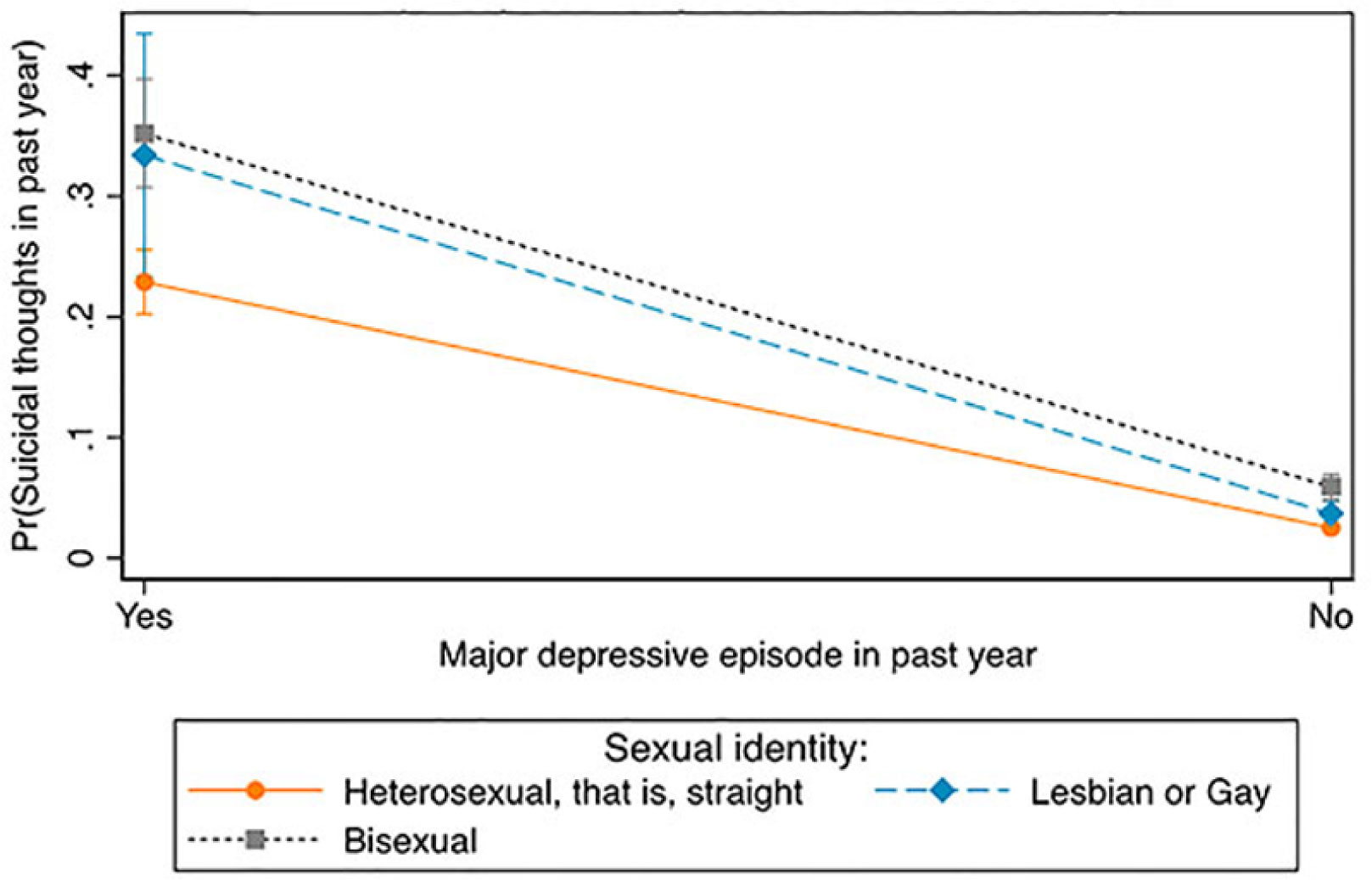
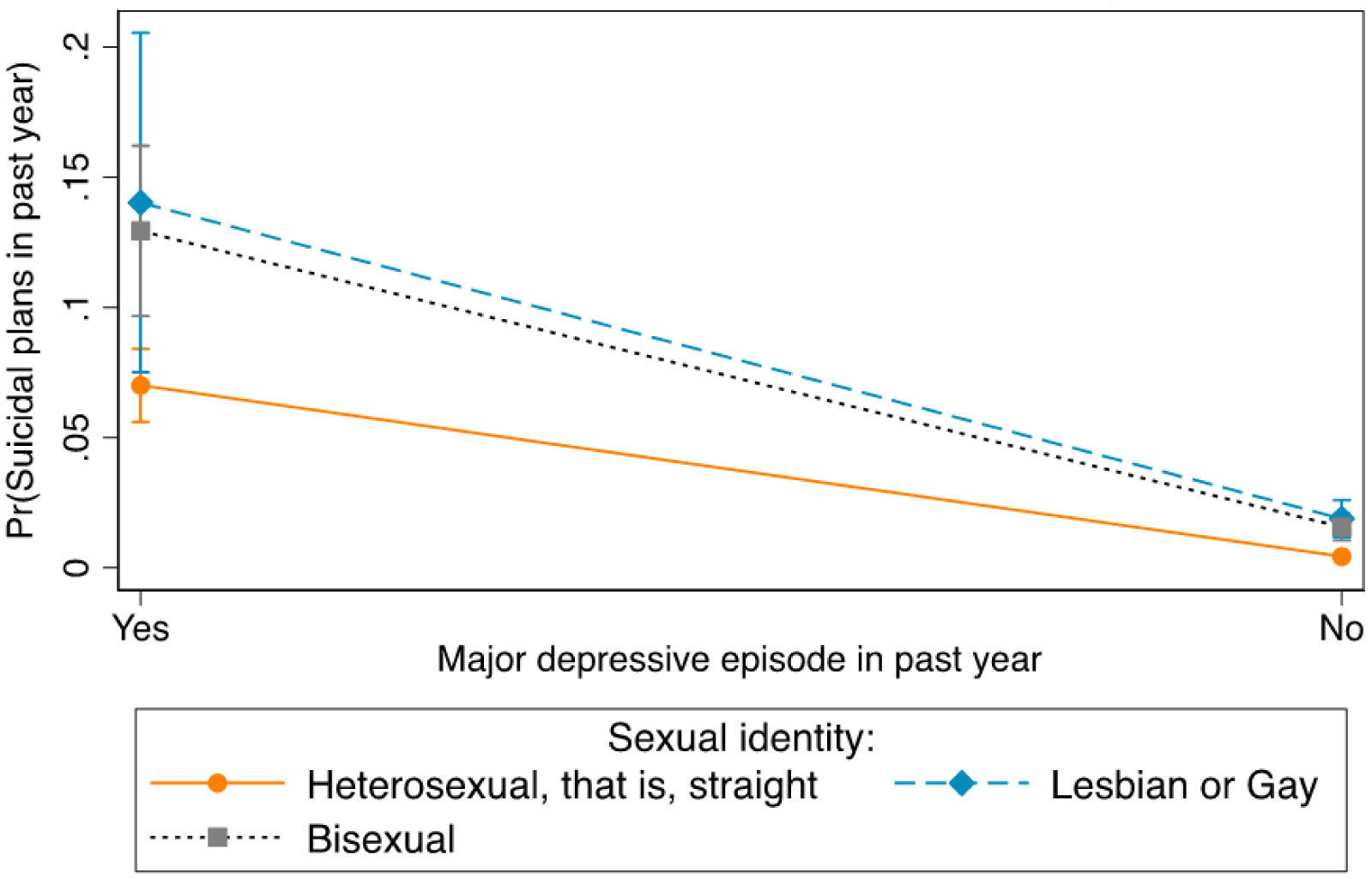
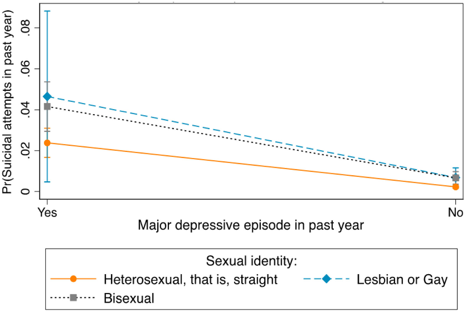
About 4.89%, 1.37%, and 0.56% of the population experienced suicidal thoughts, plans, and attempts, respectively. Those aged 18–25 years old had a higher odds of suicidality compared to those aged 26 years or older. Compared to those who reported having no alcohol use dependence, illicit drug use dependence, and major depressive episodes (MDEs), those who reported alcohol use dependence, illicit drug use dependence, and MDE had higher odds of suicidal thoughts, plans, and attempts. Between all sexual identity groups, bisexuals who experienced MDEs had the highest probability of having suicidal thoughts while lesbians and gays who experienced MDE showed a higher probability of suicidal plans and attempts compared to heterosexuals. Within each sexual identity group, the probability of having suicidal thoughts, suicidal plans, and suicidal attempts was higher for those who had experienced MDEs compared to those who had not experienced MDEs.
Substance use disorder and MDE symptoms were associated with increased suicidality, especially among young adults and sexual minority people. This disparity underscores the need for tailored interventions and policies to enhance the provision of prompt mental health screening, diagnosis, and linkage to care for mental health services, particularly among the most vulnerable in the population.
Citation: David Adzrago, Ikponmwosa Osaghae, Nnenna Ananaba, Sylvia Ayieko, Pierre Fwelo, Nnabuchi Anikpezie, Donna Cherry. Examining differences in suicidality between and within mental health disorders and sexual identity among adults in the United States[J]. AIMS Public Health, 2021, 8(4): 636-654. doi: 10.3934/publichealth.2021051
Suicide is a leading but preventable cause of death and is preceded by domains of thoughts, plans, and attempts. We assessed the prevalence of suicidality domains and determined the association of suicidality domains with sexual identity, mental health disorder symptoms, and sociodemographic characteristics.
We used the 2019 National Survey on Drug Use and Health (NSDUH) data to perform weighted multivariable logistic regression and margins analyses to examine between and within-group differences in suicidality by sexual identity among adults aged ≥ 18 years.
About 4.89%, 1.37%, and 0.56% of the population experienced suicidal thoughts, plans, and attempts, respectively. Those aged 18–25 years old had a higher odds of suicidality compared to those aged 26 years or older. Compared to those who reported having no alcohol use dependence, illicit drug use dependence, and major depressive episodes (MDEs), those who reported alcohol use dependence, illicit drug use dependence, and MDE had higher odds of suicidal thoughts, plans, and attempts. Between all sexual identity groups, bisexuals who experienced MDEs had the highest probability of having suicidal thoughts while lesbians and gays who experienced MDE showed a higher probability of suicidal plans and attempts compared to heterosexuals. Within each sexual identity group, the probability of having suicidal thoughts, suicidal plans, and suicidal attempts was higher for those who had experienced MDEs compared to those who had not experienced MDEs.
Substance use disorder and MDE symptoms were associated with increased suicidality, especially among young adults and sexual minority people. This disparity underscores the need for tailored interventions and policies to enhance the provision of prompt mental health screening, diagnosis, and linkage to care for mental health services, particularly among the most vulnerable in the population.

| [1] |
Naghavi M (2019) Global, regional, and national burden of suicide mortality 1990 to 2016: systematic analysis for the Global Burden of Disease Study 2016. BMJ 364: l94. doi: 10.1136/bmj.l94

|
| [2] |
Stone DM, Jones CM, Mack KA (2021) Changes in suicide rates-United States, 2018–2019. Morb Mortal Wkly Rep 70: 261-268. doi: 10.15585/mmwr.mm7008a1
|
| [3] | NIMH, Suicide Available from: https://www.nimh.nih.gov/health/statistics/suicide#. |
| [4] |
Han B, Kott PS, Hughes A, et al. (2016) Estimating the rates of deaths by suicide among adults who attempt suicide in the United States. J Psychiatr Res 77: 125-133. doi: 10.1016/j.jpsychires.2016.03.002
|
| [5] |
Baca-Garcia E, Perez-Rodriguez MM, Oquendo MA, et al. (2011) Estimating risk for suicide attempt: are we asking the right questions? Passive suicidal ideation as a marker for suicidal behavior. J Affect Disord 134: 327-332. doi: 10.1016/j.jad.2011.06.026
|
| [6] | Substance Abuse and Mental Health Services Administration (SAMHSA), 2019 NSDUH Detailed Tables. National Survey on Drug Use and Health Available from: https://www.samhsa.gov/data/report/2019-nsduh-detailed-tables. |
| [7] | Substance Abuse and Mental Health Services Administration (SAMHSA), Suicidal Thoughts and Behavior among Adults: Results from the 2015 National Survey on Drug Use and Health Available from: https://www.samhsa.gov/data/sites/default/files/NSDUH-DR-FFR3-2015/NSDUH-DR-FFR3-2015.htm. |
| [8] | Borders A (2020) Rumination and related constructs causes, consequences, and treatment of thinking too much Academic Press. |
| [9] |
Chapman AL, Dixon-Gordon KL (2007) Emotional antecedents and consequences of deliberate self-harm and suicide attempts. Suicide Life Threat Behav 37: 543-552. doi: 10.1521/suli.2007.37.5.543
|
| [10] |
Nock MK, Hwang I, Sampson NA, et al. (2010) Mental disorders, comorbidity and suicidal behavior: Results from the National Comorbidity Survey Replication. Mol Psychiatry 15: 868-876. doi: 10.1038/mp.2009.29
|
| [11] |
Klonsky ED, May AM, Saffer BY (2016) Suicide, suicide attempts, and suicidal ideation. Annu Rev Clin Psychol 12: 307-330. doi: 10.1146/annurev-clinpsy-021815-093204
|
| [12] |
Hawton K, Casañas I, Comabella C, Haw C, et al. (2013) Risk factors for suicide in individuals with depression: A systematic review. J Affective Disord 147: 17-28. doi: 10.1016/j.jad.2013.01.004
|
| [13] |
Steinhausen HC, Metzke CWW (2004) The impact of suicidal ideation in preadolescence, adolescence, and young adulthood on psychosocial functioning and psychopathology in young adulthood. Acta Psychiatr Scand 110: 438-445. doi: 10.1111/j.1600-0447.2004.00364.x
|
| [14] |
Aseltine RH, DeMartino R (2004) An outcome evaluation of the SOS Suicide Prevention Program. Am J Public Health 94: 446-451. doi: 10.2105/AJPH.94.3.446
|
| [15] | Hallfors DD, Waller MW, Ford CA, et al. (2004) Adolescent depression and suicide risk: Association with sex and drug behavior. Am J Prev Med 27: 224-231. |
| [16] |
Bolognini M, Plancherel B, Laget J, et al. (2009) Adolescent's suicide attempts: populations at risk, vulnerability, and substance use. Subst Use Misuse 38: 1651-1669. doi: 10.1081/JA-120024235
|
| [17] | Hafeez H, Zeshan M, Tahir MA, et al. (2017) Health care disparities among lesbian, gay, bisexual, and transgender youth: a literature review. Cureus 9. |
| [18] | Manalastas EJ (2013) Sexual orientation and suicide risk in the Philippines: Evidence from a nationally representative sample of young Filipino men. Philipp J Psychol 46: 1-13. |
| [19] |
Haas AP, Eliason M, Mays VM, et al. (2010) Suicide and suicide risk in lesbian, gay, bisexual, and transgender populations: Review and recommendations. J Homosexual 58: 10-51. doi: 10.1080/00918369.2011.534038
|
| [20] |
Janković J, Slijepčević V, Miletić V (2020) Depression and suicidal behavior in LGB and heterosexual populations in Serbia and their differences: Cross-sectional study. PLoS One 15: e0234188. doi: 10.1371/journal.pone.0234188
|
| [21] |
Yi H, Lee H, Park J, et al. (2017) Health disparities between lesbian, gay, and bisexual adults and the general population in South Korea: Rainbow Connection Project I. Epidemiol Health 39: e2017046. doi: 10.4178/epih.e2017046
|
| [22] |
Hottes TS, Bogaert L, Rhodes AE, et al. (2016) Lifetime prevalence of suicide attempts among sexual minority adults by study sampling strategies: A systematic review and meta-analysis. Am J Public Health 106: e1-e12. doi: 10.2105/AJPH.2016.303088
|
| [23] |
Marshal MP, Dietz LJ, Friedman MS, et al. (2011) Suicidality and depression disparities between sexual minority and heterosexual youth: A meta-analytic review. J Adolescent Health 49: 115-123. doi: 10.1016/j.jadohealth.2011.02.005
|
| [24] |
Miranda-Mendizábal A, Castellví P, Parés-Badell O, et al. (2017) Sexual orientation and suicidal behaviour in adolescents and young adults: systematic review and meta-analysis. Brit J Psychiat 211: 77-87. doi: 10.1192/bjp.bp.116.196345
|
| [25] | Substance Abuse and Mental Health Services Administration (SAMHSA), 2019 National Survey on Drug Use and Health (NSDUH): Methodological Summary and Definitions Available from: https://www.samhsa.gov/data/sites/default/files/reports/rpt29395/2019NSDUHMethodsSummDefs/2019NSDUHMethodsSummDefs082120.htm. |
| [26] | American Psychiatric Association Diagnostic and Statistical Manual of Mental Disorders (DSM-5) (2013) . |
| [27] | National Comorbidity Survey Available from: https://www.hcp.med.harvard.edu/ncs/. |
| [28] | Center for Behavioral Health Statistics and Quality 2019 National Survey on Drug Use and Health Public Use File Codebook (2020) . |
| [29] | Fauman MA (2002) Study Guide to DSM-IV-TR American Psychiatric Publishing, Inc. |
| [30] |
Williams R (2012) Using the margins command to estimate and interpret adjusted predictions and marginal effects. Stata J 12: 308-331. doi: 10.1177/1536867X1201200209
|
| [31] | Why Stata, Stata Available from: https://www.stata.com/why-use-stata/. |
| [32] |
Darvishi N, Farhadi M, Haghtalab T, et al. (2015) Alcohol-related risk of suicidal ideation, suicide attempt, and completed suicide: a meta-analysis. PloS One 10: e0126870. doi: 10.1371/journal.pone.0126870
|
| [33] |
Pompili M, Serafini G, Innamorati M, et al. (2010) Suicidal behavior and alcohol abuse. Int J Environ Res Public Health 7: 1392-1431. doi: 10.3390/ijerph7041392
|
| [34] |
De Beurs D, Have MT, Cuijpers P, et al. (2019) The longitudinal association between lifetime mental disorders and first onset or recurrent suicide ideation. BMC Psychiatry 19: 345. doi: 10.1186/s12888-019-2328-8
|
| [35] |
Too LS, Spittal MJ, Bugeja L, et al. (2019) The association between mental disorders and suicide: A systematic review and meta-analysis of record linkage studies. J Affective Disord 259: 302-313. doi: 10.1016/j.jad.2019.08.054
|
| [36] |
Brådvik L (2018) Suicide risk and mental disorders. Int J Environ Res Public Health 15: 2028. doi: 10.3390/ijerph15092028
|
| [37] |
Conner KR, Duberstein PR, Conwell Y, et al. (2003) Reactive aggression and suicide: Theory and evidence. Aggress Violent Beh 8: 413-432. doi: 10.1016/S1359-1789(02)00067-8
|
| [38] |
Ilgen MA, Bohnertet ASB, Ignacio RV, et al. (2010) Psychiatric diagnoses and risk of suicide in veterans. Arch Gen Psychiatry 67: 1152-1158. doi: 10.1001/archgenpsychiatry.2010.129
|
| [39] | The neurobiology of substance use, misuse, and addiction (2016) .Available from: https://www.ncbi.nlm.nih.gov/books/NBK424849/. |
| [40] |
Koob GF, Simon EJ (2009) The neurobiology of addiction: where we have been and where we are going. J Drug Issues 39: 115-132. doi: 10.1177/002204260903900110
|
| [41] |
Evans CJ, Cahill CM (2016) Neurobiology of opioid dependence in creating addiction vulnerability. F1000Res 5: F1000. doi: 10.12688/f1000research.8369.1
|
| [42] |
Twenge JM, Cooper AB, Joiner TE, et al. (2019) Age, period, and cohort trends in mood disorder indicators and suicide-related outcomes in a nationally representative dataset, 2005–2017. J Abnorm Psychol 128: 185-199. doi: 10.1037/abn0000410
|
| [43] |
Ohayon MM, Schatzberg AF (2002) Prevalence of depressive episodes with psychotic features in the general population. Am J Psychiatry 159: 1855-1861. doi: 10.1176/appi.ajp.159.11.1855
|
| [44] | Perez-Rodriguez MM, Baca-Garcia E, Oquendo MA, et al. (2008) Ethnic differences in suicidal ideation and attempts. Primary Psychiatry 15: 44. |
| [45] |
Utsey SO, Hook JN, Stanard P (2007) A re-examination of cultural factors that mitigate risk and promote resilience in relation to African American suicide: A review of the literature and recommendations for future research. Death Stud 31: 399-416. doi: 10.1080/07481180701244553
|
| [46] |
Compton MT, Thompson NJ, Kaslow NJ (2005) Social environment factors associated with suicide attempt among low-income African Americans: The protective role of family relationships and social support. Soc Psychiatry Psychiatr Epidemiol 40: 175-185. doi: 10.1007/s00127-005-0865-6
|
| [47] |
Rosoff DB, Kaminsky ZA, McIntosh AM, et al. (2020) Educational attainment reduces the risk of suicide attempt among individuals with and without psychiatric disorders independent of cognition: a bidirectional and multivariable Mendelian randomization study with more than 815,000 participants. Transl Psychiatry 10: 388. doi: 10.1038/s41398-020-01047-2
|
| [48] |
Lynch KE, Gatsby E, Viernes B, et al. (2020) Evaluation of suicide mortality among sexual minority US veterans from 2000 to 2017. JAMA Netw Open 3: e2031357. doi: 10.1001/jamanetworkopen.2020.31357
|
| [49] |
Mustanski BS, Garofalo R, Emerson EM (2011) Mental health disorders, psychological distress, and suicidality in a diverse sample of lesbian, gay, bisexual, and transgender youths. Am J Public Health 100: 2426-2432. doi: 10.2105/AJPH.2009.178319
|
| [50] |
Noell JW, Ochs LM (2001) Relationship of sexual orientation to substance use, suicidal ideation, suicide attempts, and other factors in a population of homeless adolescents. J Adolesc Health 29: 31-36. doi: 10.1016/S1054-139X(01)00205-1
|
| [51] | Alessi EJ, Greenfield B, Manning D, et al. (2020) Victimization and resilience among sexual and gender minority homeless youth engaging in survival sex. J Interpers Violence 0886260519898434. |
| [52] |
Jenkins R, Kovess V (2002) Evaluation of suicide prevention: a European approach. Int Rev Psychiatr 14: 34-41. doi: 10.1080/09540260120114041
|
Figures(3) / Tables(2)

David Adzrago, Ikponmwosa Osaghae, Nnenna Ananaba, Sylvia Ayieko, Pierre Fwelo, Nnabuchi Anikpezie, Donna Cherry. Examining differences in suicidality between and within mental health disorders and sexual identity among adults in the United States[J]. AIMS Public Health, 2021, 8(4): 636-654. doi: 10.3934/publichealth.2021051


 DownLoad: