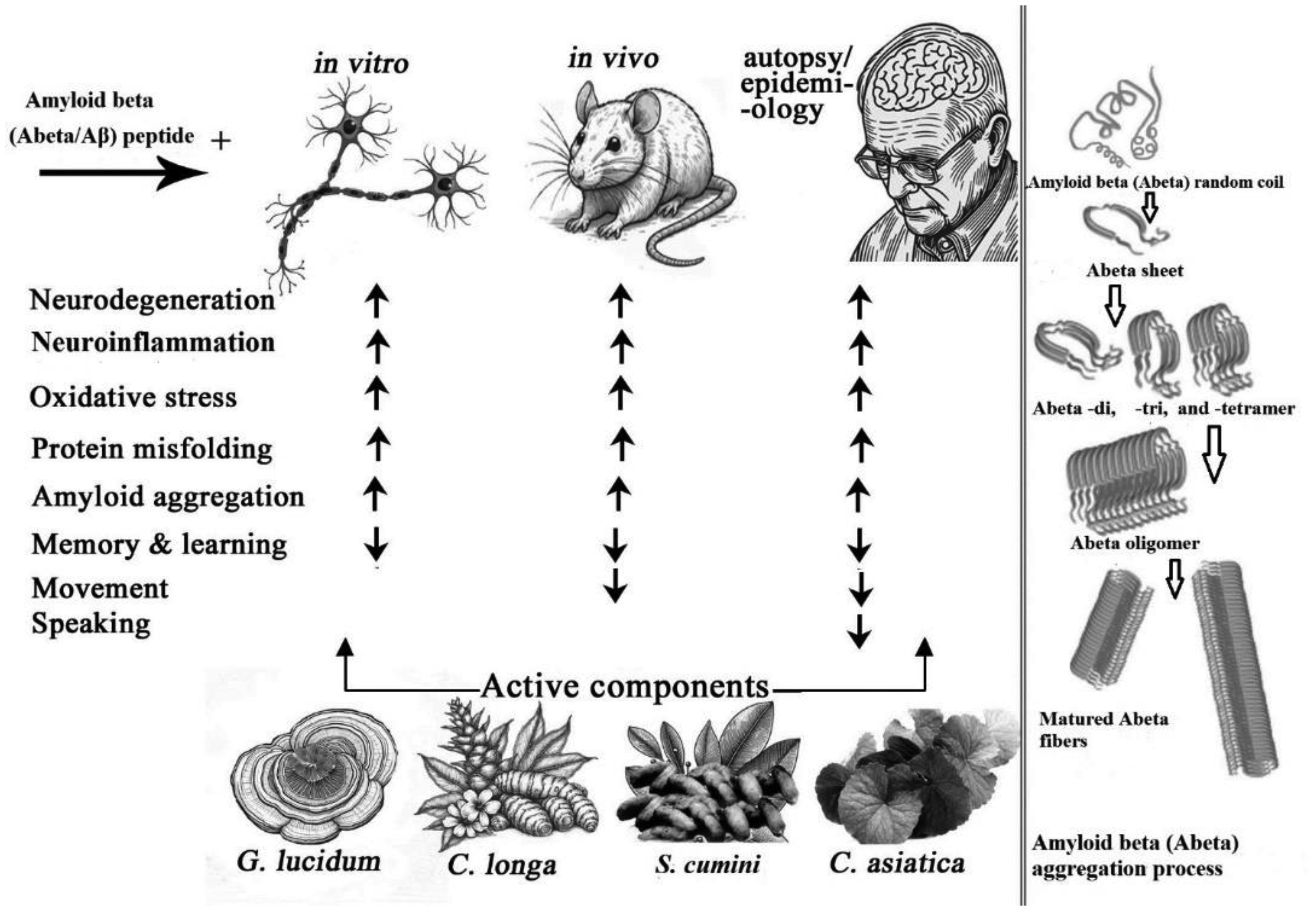
Alzheimer's disease (AD), a neurodegenerative disease (ND), has been plaguing healthcare and health policy agencies due to its ever-soaring impact globally. It is timely to develop appropriate measures to combat global AD burden. Due to structural and functional similarity, rodent models offer the best alternative to study AD pathogenesis and therapeutics. In this special issue, the present article reviews the state-of-the-art findings on AD model animals from the alternative and integrative medicinal point of view. Our integrative therapeutic agents include fungi (Ganoderma lucidum), turmeric (Curcuma longa), Indian black berry (black plum, jamun) (Syzygium cumini), and madecassoside (derived from Centella asiatica). Their bio-components, especially flavonoids, polyphenols, and tri-terpenoids, resist oxidative stress, amyloid beta fibrillation, and pro-inflammatory cytokine levels; improve anti-oxidative prowess; and improve learning-related memory and anxiety-like behavior in AD model animals. Most of the findings described here are outcomes of our own studies. However, our claims have been substantiated with evidence from some other studies in the relevant field. As a whole, integrative medicinal approaches towards AD pathogenesis using these natural products seem promising in AD protection.
Citation: Shahdat Hossain, Mohammad Azizur Rahman, Shoriful Islam Joy, Anuradha Baraik, Shadman Nazib. Integrative medicinal approaches towards Alzheimer's disease model animals–A new hope[J]. AIMS Molecular Science, 2024, 11(3): 221-230. doi: 10.3934/molsci.2024013
Alzheimer's disease (AD), a neurodegenerative disease (ND), has been plaguing healthcare and health policy agencies due to its ever-soaring impact globally. It is timely to develop appropriate measures to combat global AD burden. Due to structural and functional similarity, rodent models offer the best alternative to study AD pathogenesis and therapeutics. In this special issue, the present article reviews the state-of-the-art findings on AD model animals from the alternative and integrative medicinal point of view. Our integrative therapeutic agents include fungi (Ganoderma lucidum), turmeric (Curcuma longa), Indian black berry (black plum, jamun) (Syzygium cumini), and madecassoside (derived from Centella asiatica). Their bio-components, especially flavonoids, polyphenols, and tri-terpenoids, resist oxidative stress, amyloid beta fibrillation, and pro-inflammatory cytokine levels; improve anti-oxidative prowess; and improve learning-related memory and anxiety-like behavior in AD model animals. Most of the findings described here are outcomes of our own studies. However, our claims have been substantiated with evidence from some other studies in the relevant field. As a whole, integrative medicinal approaches towards AD pathogenesis using these natural products seem promising in AD protection.

| [1] |
Gitler AD, Dhillon P, Shorter J (2017) Neurodegenerative disease: Models, mechanisms, and a new hope. Dis Model Mech 10: 499-502. https://doi.org/10.1242/dmm.030205 
|
| [2] |
Dhapola R, Kumari S, Sharma P, et al. (2023) Insight into the emerging and common experimental in-vivo models of Alzheimer's disease. Lab Anim Res 39: 33. https://doi.org/10.1186/s42826-023-00184-1
|
| [3] |
Dawson TM, Golde TE, Tourenne C (2018) Animal models of neurodegenerative diseases. Nat Neurosci 21: 1370-1379. https://doi.org/10.1038/s41593-018-0236-8
|
| [4] |
Nabeshima T, Nitta A (1994) Memory impairment and neuronal dysfunction induced by beta-amyloid protein in rats. Tohoku J Exp Med 174: 241-249. https://doi.org/10.1620/tjem.174.241
|
| [5] |
Lyketsos CG, Carrillo MC, Ryan JM, et al. (2011) Neuropsychiatric symptoms in Alzheimer's disease. Alzheimers Dement 7: 532-539. https://doi.org/10.1016/j.jalz.2011.05.2410
|
| [6] |
Sadigh-Eteghad S, Sabermarouf B, Majdi A, et al. (2015) Amyloid-beta: A crucial factor in Alzheimer's disease. Med Princ Pract 24: 1-10. https://doi.org/10.1159/000369101
|
| [7] | Alzheimer's association.Alzheimer's association report: 2019 Alzheimer's disease facts and figures. Alzheimer's Dement (2019) 15: 321-387. https://doi.org/10.1016/j.jalz.2019.01.010 |
| [8] | Rahman MA, Alpona AK, Biswas D, et al. (2023) Neuronal malady in epileptic brain–Amendment with mushrooms. Arch Neurol Neurosci 14: 2023. http://doi.org/10.33552/ANN.2023.14.000847 |
| [9] |
Rahman MA, Hossain S, Abdullah N, et al. (2020) Ganoderma lucidum modulates neuronal distorted cytoskeletal proteomics and protein-protein interaction in Alzheimer's disease model animals. Arch Neurol Neurosci 9: 2020. http://doi.org/10.33552/ANN.2020.09.000713
|
| [10] |
Sharma P., Tulsawani R. (2020) Ganoderma lucidum aqueous extract prevents hypobaric hypoxia induced memory deficit by modulating neurotransmission, neuroplasticity and maintaining redox homeostasis. Sci Rep 10: 8944. https://doi.org/10.1038/s41598-020-65812-5
|
| [11] | Rahman MA, Hossain S, Abdullah N, et al. (2020) Validation of Ganoderma lucidum against hypercholesterolemia and Alzheimer's disease. Eur J Biol Res 10: 314-325. http://doi.org/10.5281/zenodo.4009588 |
| [12] | Rahman MA, Hossain S, Abdullah N, et al. (2020) Ganoderma lucidum ameliorates spatial memory and memory-related protein markers in hypercholesterolemic and Alzheimer's disease model rats. Arch Neurol Neurol Disord 3: 117-129. |
| [13] |
Rahman MA, Hossain S, Abdullah N, et al. (2020) Lingzhi or Reishi medicinal mushroom, Ganoderma lucidum (Agaricomycetes) ameliorates non-spatial learning and memory deficits in rats with hypercholesterolemia and Alzheimer's disease. Int J Med Mushroom 22: 93-103. http://doi.org/10.1615/IntJMedMushrooms.2020033383
|
| [14] |
Rahman MA, Hossain S, Abdullah N, et al. (2019) Brain proteomics links oxidative stress with metabolic and cellular stress response proteins in behavioural alteration of Alzheimer's disease model rats. AIMS Neurosci 6: 299-315. http://doi.org/10.3934/Neuroscience.2019.4.299
|
| [15] |
Zhang Y, Song S, Li H, et al. (2022) Polysaccharide from Ganoderma lucidum alleviates cognitive impairment in a mouse model of chronic cerebral hypoperfusion by regulating CD4+ CD25+ Foxp3+ regulatory T cells. Food Funct 13: 1941-1952. http://doi.org/10.1039/d1fo03698j
|
| [16] |
Huang S, Mao J, Ding K, et al. (2017) Polysaccharides from Ganoderma lucidum promote cognitive function and neural progenitor proliferation in mouse model of Alzheimer's disease. Stem Cell Reports 8: 84-94. http://doi.org/10.1016/j.stemcr.2016.12.007
|
| [17] |
Cai Q, Li Y, Pei G (2017) Polysaccharides from Ganoderma lucidum attenuate microglia-mediated neuroinflammation and modulate microglial phagocytosis and behavioural response. J Neuroinflammation 14: 63. http://doi.org/10.1186/s12974-017-0839-0
|
| [18] |
Zhang Y, Wang X, Yang X, et al. (2021) Ganoderic acid A to alleviate neuroinflammation of Alzheimer's disease in mice by regulating the imbalance of the Th17/Tregs axis. J Agric Food Chem 69: 14204-14214. http://doi.org/10.1021/acs.jafc.1c06304
|
| [19] |
Lai G, Guo Y, Chen D, et al. (2019) Alcohol extracts from Ganoderma lucidum delay the progress of Alzheimer's Disease by regulating DNA methylation in rodents. Front Pharmacol 10: 272. http://doi.org/10.3389/fphar.2019.00272
|
| [20] |
Ahmad F, Singh G, Soni H, et al. (2022) Identification of potential neuroprotective compound from Ganoderma lucidum extract targeting microtubule affinity regulation kinase 4 involved in Alzheimer's disease through molecular dynamics simulation and MMGBSA. Aging Med (Milton) 6: 144-154. http://doi.org/10.1002/agm2.12232
|
| [21] |
Zeng M, Qi L, Guo Y, et al. (2021) Long-term administration of triterpenoids from Ganoderma lucidum mitigates age-associated brain physiological decline via regulating sphingolipid metabolism and enhancing autophagy in mice. Front Aging Neurosci 13: 628860. https://doi.org/10.3389/fnagi.2021.628860
|
| [22] |
Jeong JH, Hong GL, Jeong YG, et al. (2023) Mixed medicinal mushroom mycelia attenuates Alzheimer's disease pathologies in vitro and in vivo. Curr Issues Mol Biol 45: 6775-6789. https://doi.org/10.3390/cimb45080428
|
| [23] |
Khatian N, Aslam M (2019) Effect of Ganoderma lucidum on memory and learning in mice. Clin Phytosci 5: 4. https://doi.org/10.1186/s40816-019-0101-7
|
| [24] |
Sharma P, Tulsawani R (2020) Ganoderma lucidum aqueous extract prevents hypobaric hypoxia induced memory deficit by modulating neurotransmission, neuroplasticity and maintaining redox homeostasis. Sci Rep 10: 8944. https://doi.org/10.1038/s41598-020-65812-5
|
| [25] |
Silva AM, Preto M, Grosso C, et al. (2023) Tracing the path between mushrooms and Alzheimer's disease—A literature review. Molecules 28: 5614. https://doi.org/10.3390/molecules28145614
|
| [26] |
Tran YH, Nguyen TTT, Nguyen PT, et al. (2021) Effects of Ganoderma Lucidum extract on morphine-induced addiction and memory impairment in mice. Biointerface Res Appl Chem 12: 1076-1084. https://doi.org/10.33263/BRIAC121.10761084
|
| [27] | Rezvanirad A, Mardani M, Shirzad H, et al. (2016) Curcuma longa: A review of therapeutic effects in traditional and modern medical references. J Chem Pharmac Sci 9: 3438-4348. |
| [28] |
Chen M, Du ZY, Zheng X, et al. (2018) Use of curcumin in diagnosis, prevention, and treatment of Alzheimer's disease. Neural Regen Res 13: 742-752. https://doi.org/10.4103/1673-5374.230303
|
| [29] |
da Costa IM, de Moura Freire MA, de Paiva Cavalcanti JRL, et al. (2019) Supplementation with curcuma longa reverses neurotoxic and behavioral damage in models of Alzheimer's disease: A systematic review. Curr Neuropharmacol 17: 406-421. https://doi.org/10.2174/0929867325666180117112610
|
| [30] |
Chen MH, Chiang BH (2020) Modification of curcumin-loaded liposome with edible compounds to enhance ability of crossing blood brain barrier. Colloid Surfaces A 599: 124862. https://doi.org/10.1016/j.colsurfa.2020.124862
|
| [31] | Liu ZJ, Li ZH, Liu L, et al. (2016) Curcumin attenuates beta-amyloid-induced neuroinflammation via activation of peroxisome proliferator-activated receptor-gamma function in a rat model of Alzheimer's disease. Front Pharmacol 7: 261. https://doi.org/10.3389/fphar.2016.00261 |
| [32] | Ringman JM, Frautschy SA, Teng E, et al. (2012) Oral curcumin for Alzheimer's disease: Tolerability and efficacy in a 24-week randomized, double blind, placebo-controlled study. Alz Res Therapy 43: 4. https://doi.org/10.1186/alzrt146 |
| [33] |
Assi AA, Farrag MMY, Badary DM, et al. (2023) Protective effects of curcumin and Ginkgo biloba extract combination on a new model of Alzheimer's disease. Inflammopharmacology 31: 1449-1464. https://doi.org/10.1007/s10787-023-01164-6
|
| [34] |
Park SY, Kim DSHL (2002) Discovery of natural products from Curcuma longa that protect cells from beta-amyloid insult: A drug discovery effort against Alzheimer's disease. J Nat Prod 65: 1227-1231. https://doi.org/10.1021/np010039x
|
| [35] |
do Nascimento-Silva NR, Bastos RP, da Silva FA (2022) Jambolan (Syzygium cumini (L.) Skeels): A review on its nutrients, bioactive compounds and health benefits. J Food Compos Anal 109: 104491. https://doi.org/10.1016/j.jfca.2022.104491
|
| [36] | Hossain S, Islam J, Bhowmick S, et al. (2017) Effects of Syzygium cumini seed extract on the memory loss of Alzheimer's disease model rats. Adv Alzh Dis 6: 53-73. https://doi.org/10.4236/aad.2017.63005 |
| [37] |
Malik N, Javaid S, Ashraf W, et al. (2023) Long-term supplementation of Syzygium cumini (L.) skeels concentrate alleviates age-related cognitive deficit and oxidative damage: A comparative study of young vs. old mice. Nutrients 15: 666. https://doi.org/10.3390/nu15030666
|
| [38] |
Amir Rawa MS, Mazlan MKN, Ahmad R, et al. (2022) Roles of syzygium in anti-cholinesterase, anti-diabetic, anti-inflammatory, and antioxidant: From Alzheimer's perspective. Plants 11: 1476. https://doi.org/10.3390/plants11111476
|
| [39] | Basiru OA, Ojo OA, Akuboh OS, et al. (2017) The protective effect of polyphenol-rich extract of Syzygium cumini leaves on cholinesterase and brain antioxidant status in alloxan-induced diabetic rats. Jordan J Biol Sci 11: 163-169. |
| [40] |
Hawash ZAS, Yassien EM, Alotaibi BS, et al. (2023) Assessment of anti-Alzheimer pursuit of jambolan fruit extract and/or choline against AlCl3 toxicity in rats. Toxics 11: 509. https://doi.org/10.3390/toxics11060509
|
| [41] |
Mujawah A, Rauf A, Bawazeer S, et al. (2023) Isolation, structural elucidation, in vitro anti-α-glucosidase, anti-β-secretase, and in silico studies of bioactive compound isolated from Syzygium cumini L. Processes 11: 880. https://doi.org/10.3390/pr11030880
|
| [42] | Al Mamun A, Hashimoto M, Katakura M, et al. (2014) Neuroprotective effect of madecassoside evaluated using amyloid β1-42-mediated in vitro and in vivo Alzheimer's disease models. Int J. Indigen Med Plants 47: 1669-1682. |
| [43] | Mamun AA, Hashimoto M, Hossain S, et al. (2015) Confirmation of the experimentally-proven therapeutic utility of madecassoside in an Aβ1-42 infusion rat model of Alzheimer's disease by in silico analyses. Adv Alz Dis 4: 37-44. https://doi.org/10.4236/aad.2015.42005 |
| [44] |
Ling Z, Zhou S, Zhou Y, et al. (2024) Protective role of madecassoside from Centella asiatica against protein L-isoaspartyl methyltransferase deficiency-induced neurodegeneration. Neuropharmacology 246: 109834. https://doi.org/10.1016/j.neuropharm.2023.109834
|
Figures(1)

Shahdat Hossain, Mohammad Azizur Rahman, Shoriful Islam Joy, Anuradha Baraik, Shadman Nazib. Integrative medicinal approaches towards Alzheimer's disease model animals–A new hope[J]. AIMS Molecular Science, 2024, 11(3): 221-230. doi: 10.3934/molsci.2024013


 DownLoad: