A truncation mutation in the <i>L1CAM</i> gene in a child with hydrocephalus

Madhan Srinivasamurthy; Nagaraj Kakanahalli; Shreeshail V. Benakanal; Madhan Srinivasamurthy; Nagaraj Kakanahalli; Shreeshail V. Benakanal

doi:10.3934/molsci.2021017

AIMS Molecular Science

2021, Volume 8, Issue 4: 223-232. doi: 10.3934/molsci.2021017

Previous Article Next Article

Research article

A truncation mutation in the L1CAM gene in a child with hydrocephalus

1.
Molecular Genetics Laboratory, Department of Applied Zoology, Kuvempu University, Jnanasahyadri, Shankaraghatta, Shivamogga, Karnataka, 577451, India
2.
Department of Paediatrics, Shivamogga Institute of Medical Sciences (SIMS), Shivamogga, Karnataka, 577201, India

Received: 28 July 2021 Accepted: 14 September 2021 Published: 11 October 2021

Hydrocephalus is a neurodevelopmental, X-linked recessive disorder caused by mutations in the L1CAM gene. The L1CAM gene encodes for L1CAM protein which is essential for the nervous system development including adhesion between neurons, Myelination, Synaptogenesis etc. Herein, the present study has reported mutations in L1 syndrome patient with Hydrocephalus and Adducted thumb. Genomic DNA was extracted from patients whole blood (n = 18). The 11 exons of the L1CAM gene were amplified using specific PCR primers. The sequenced data was analysed and the pathogenicity of the mutation was predicted using the various bioinformatics programs: PROVEAN, PolyPhen2, and MUpro. The results revealed that the proband described here had nonsense mutation G1120→T at position 1120 in exon 9 which is in extracellular immunoglobulin domain (Ig4) of the L1CAM gene. This nonsense mutation is found to be truncated with a deleterious effect on developing brain of the child, and this is the first report of this novel mutation in patient with X-linked Hydrocephalus in India.
- L1CAM,
- hydrocephalus,
- adducted thumb,
- X-linked recessive,
- nonsense mutation
Citation: Madhan Srinivasamurthy, Nagaraj Kakanahalli, Shreeshail V. Benakanal. A truncation mutation in the L1CAM gene in a child with hydrocephalus[J]. AIMS Molecular Science, 2021, 8(4): 223-232. doi: 10.3934/molsci.2021017

Related Papers:

Abstract

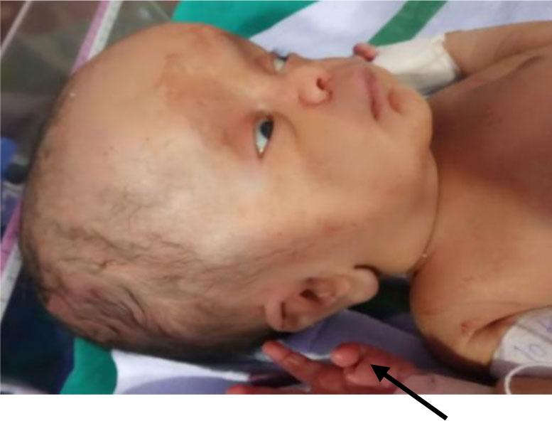
Hydrocephalus is a neurodevelopmental, X-linked recessive disorder caused by mutations in the L1CAM gene. The L1CAM gene encodes for L1CAM protein which is essential for the nervous system development including adhesion between neurons, Myelination, Synaptogenesis etc. Herein, the present study has reported mutations in L1 syndrome patient with Hydrocephalus and Adducted thumb. Genomic DNA was extracted from patients whole blood (n = 18). The 11 exons of the L1CAM gene were amplified using specific PCR primers. The sequenced data was analysed and the pathogenicity of the mutation was predicted using the various bioinformatics programs: PROVEAN, PolyPhen2, and MUpro. The results revealed that the proband described here had nonsense mutation G1120→T at position 1120 in exon 9 which is in extracellular immunoglobulin domain (Ig4) of the L1CAM gene. This nonsense mutation is found to be truncated with a deleterious effect on developing brain of the child, and this is the first report of this novel mutation in patient with X-linked Hydrocephalus in India.

Acknowledgments

We are thankful to the University Grants Commission (F. No. 41-95/2012 SR), New Delhi, India, for financial support. The proposal for this study was approved by the Institutional Ethical Committee of the University (No. KU/IEC/05-09/2014-15).

Conflict of interest

The authors declare no conflict of interest for this study.

References

[1]	Bickers D, Adams R (1949) Hereditary stenosis of the aqueduct of Sylvius as a cause of congenital hydrocephalus. Brain 72: 246-262. doi: 10.1093/brain/72.2.246
[2]	Finckh U, Schroder J, Ressler B, et al. (2000) Spectrum and detection rate of L1CAM mutations in isolated and familial cases with clinically suspected L1-disease. Am J Med Genet 92: 40-46. doi: 10.1002/(SICI)1096-8628(20000501)92:1<40::AID-AJMG7>3.0.CO;2-R
[3]	Fransen E, Camp GV, Vits L, et al. (1997) L1-associated diseases: clinical genetics divide, molecular genetics unite. Hum Mol Genet 6: 1625-1632. doi: 10.1093/hmg/6.10.1625
[4]	Samatov TR, Wicklein D, Tonevitsky AG (2016) L1CAM: Cell adhesion and more. Prog Histochem Cytochem 51: 25-32. doi: 10.1016/j.proghi.2016.05.001
[5]	Kamiguchi H, Hlavin ML, Lemmon V (1998) Role of L1 in Neural Development: What the Knockouts Tell Us. Mol Cell Neurosci 12: 48-55. doi: 10.1006/mcne.1998.0702
[6]	Moos M, Tacke R, Scherer H, et al. (1988) Neural Adhesion Molecule L1 as a Member of the Immunoglobulin Superfamily with Binding Domains Similar to Fibronectin. Nature 334: 701-703. doi: 10.1038/334701a0
[7]	Mikulak J, Negrini S, Klajn A, et al. (2012) Dual REST-dependence of L1CAM: from gene expression to alternative splicing governed by Nova2 in neural cells. J Neurochem 120: 699-709. doi: 10.1111/j.1471-4159.2011.07626.x
[8]	Bertolin C, Boaretto F, Barbon G, et al. (2010) Novel mutations in the L1CAM gene support the complexity of L1 syndrome. J Neurosci 294: 124-126.
[9]	Okamoto N, Del Maestro R, Valero R, et al. (2004) Hydrocephalus and Hirschsprung's disease with a mutation of L1CAM. J Hum Genet 49: 334-337. doi: 10.1007/s10038-004-0153-4
[10]	Vos YJ, De Walle HE, Bos KK, et al. (2010) Genotype-phenotype correlations in L1 syndrome: a guide for genetic counseling and mutation analysis. J Med Genet 47: 169-175. doi: 10.1136/jmg.2009.071688
[11]	L1CAM mutation database Available from: http://www.l1cammutationdatabase.info/default.aspx.
[12]	Kanemura Y, Takuma Y, Kamiguchi H, et al. (2005) First case of L1CAM gene mutation identified in MASA syndrome in Asia. Congenital Anomalies 45: 67-69. doi: 10.1111/j.1741-4520.2005.00067.x
[13]	Marin R, Ley-Martos M, Gutierrez G, et al. (2015) Three cases with L1 syndrome and two novel mutations in the L1CAM gene. Eur J Pediatr 174: 1541-1544. doi: 10.1007/s00431-015-2560-2
[14]	Ochando I, Vidal V, Gascon J, et al. (2015) Prenatal diagnosis of X-linked hydrocephalus in a family with a novel mutation in L1CAM gene. J Obstet Gynaecol 36: 403-405. doi: 10.3109/01443615.2015.1086982
[15]	Silan F, Ozdemir I, Lissens W (2005) A novel L1CAM mutation with L1 spectrum disorders. Prenat Diagn 25: 57-59. doi: 10.1002/pd.978
[16]	Camp GV, Vits L, Coucke P, et al. (1993) A Duplication in the L1CAM Gene Associated with X-Linked Hydrocephalus. Nat Genet 4: 421-425. doi: 10.1038/ng0893-421
[17]	Fransen E, Lemmon V, Camp VG, et al. (1995) CRASH syndrome: clinical spectrum of corpus callosum hypoplasia, retardation, adducted thumbs, spastic paraparesis and hydrocephalus due to mutations in one single gene, L1. Eur J Hum Genet 3: 273-284. doi: 10.1159/000472311
[18]	Swarna M, Sujatha M, Usha Rani P, et al. (2004) Detection of L1 CAM mutation in a male child with Mental retardation. Indian J Clin Biochem 19: 163-167. doi: 10.1007/BF02894278
[19]	Jharna P, Hemabindu L, Siva Prasad S, et al. (2006) Detection of L1 (CAM) mutations in X-linked mental retardation: A study from Andhra Pradesh, India. Indian J Hum Genet 12: 82-85. doi: 10.4103/0971-6866.27791
[20]	QIAamp DNA Mini Blood Mini Handbook Available from: https://www.qiagen.com/us/resources/resourcedetail?id=62a200d6-faf4-469b-b50f-2b59cf738962&lang=en.
[21]	NCBI Primer-Blast Available from: https://www.ncbi.nlm.nih.gov/tools/primer-blast/.
[22]	BioEdit tool Available from: http://www.mbio.ncsu.edu/BioEdit/bioedit.html.
[23]	Rosenthal A, Jouet M, Kenwrick S (1992) Aberrant splicing of neural cell adhesion molecule L1 mRNA in a family with X-linked hydrocephalus. Nat Genet 2: 107-112. doi: 10.1038/ng1092-107
[24]	Fransen E, Camp GV, Hooge RD, et al. (1998) Genotype-phenotype correlation in L1 associated diseases. J Med Genet 35: 399-404. doi: 10.1136/jmg.35.5.399
[25]	Yamasaki M, Thompson P, Lemmon V (1997) CRASH syndrome: mutations in L1CAM correlate with severity of the disease. Neuropediatrics 28: 175-178. doi: 10.1055/s-2007-973696
[26]	De Angelis E, Watkins A, Schafer M, et al. (2002) Disease-Associated Mutations in L1CAM Interfere with Ligand Interactions and Cell-Surface Expression. Hum Mol Genet 11: 1-12. doi: 10.1093/hmg/11.1.1
[27]	Kaepernick L, Legius E, Higgins J, et al. (1994) Clinical aspects of the MASA syndrome in a large family, including expressing females. Clin Genet 45: 181-185. doi: 10.1111/j.1399-0004.1994.tb04019.x
[28]	Betts MJ, Russell RB (2003) Amino acid properties and consequences of substitutions. Bioinf Genet 14: 289-316.

Reader Comments

Your name:*

Email:*
© 2021 the Author(s), licensee AIMS Press. This is an open access article distributed under the terms of the Creative Commons Attribution License (http://creativecommons.org/licenses/by/4.0)