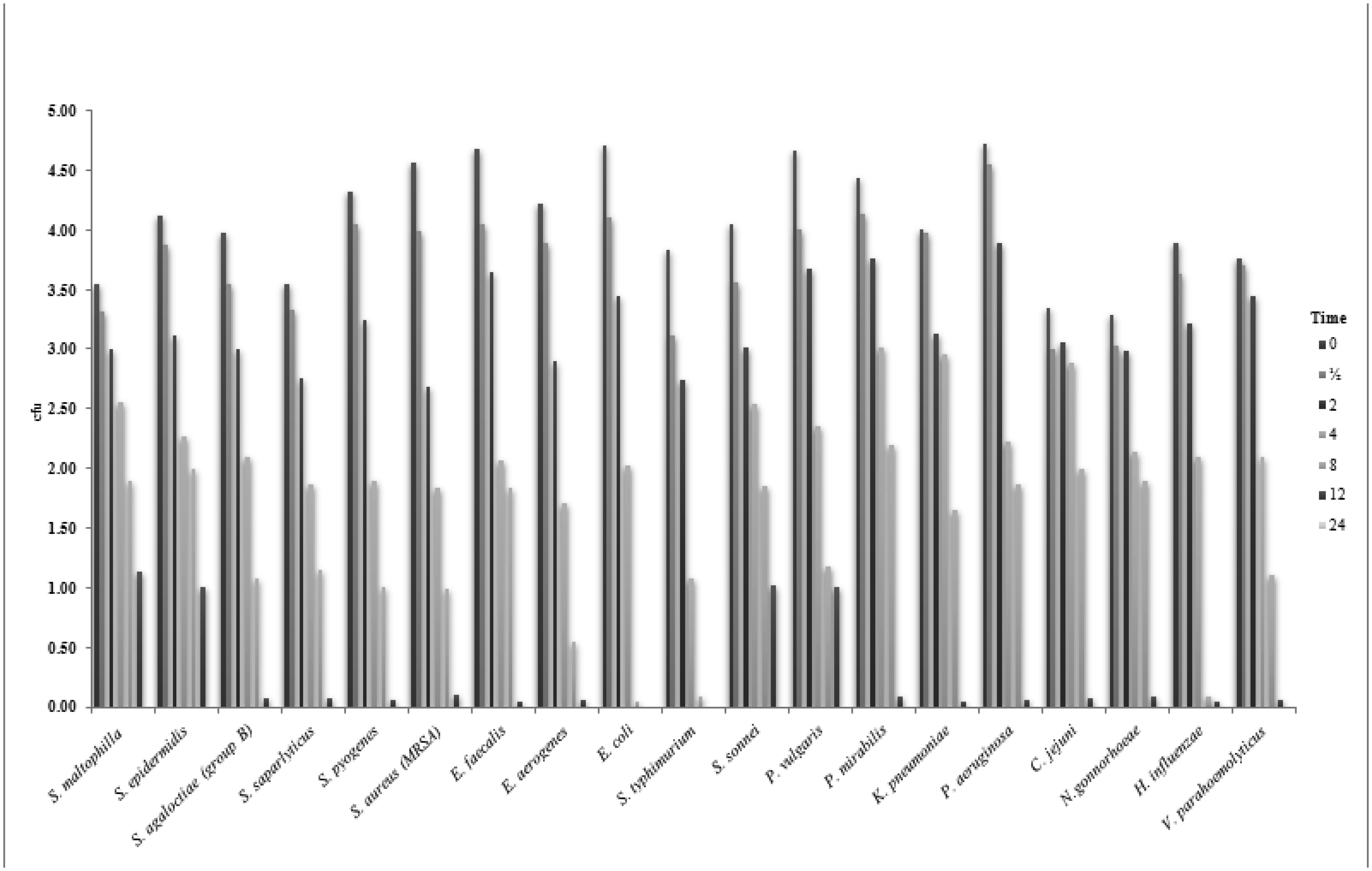
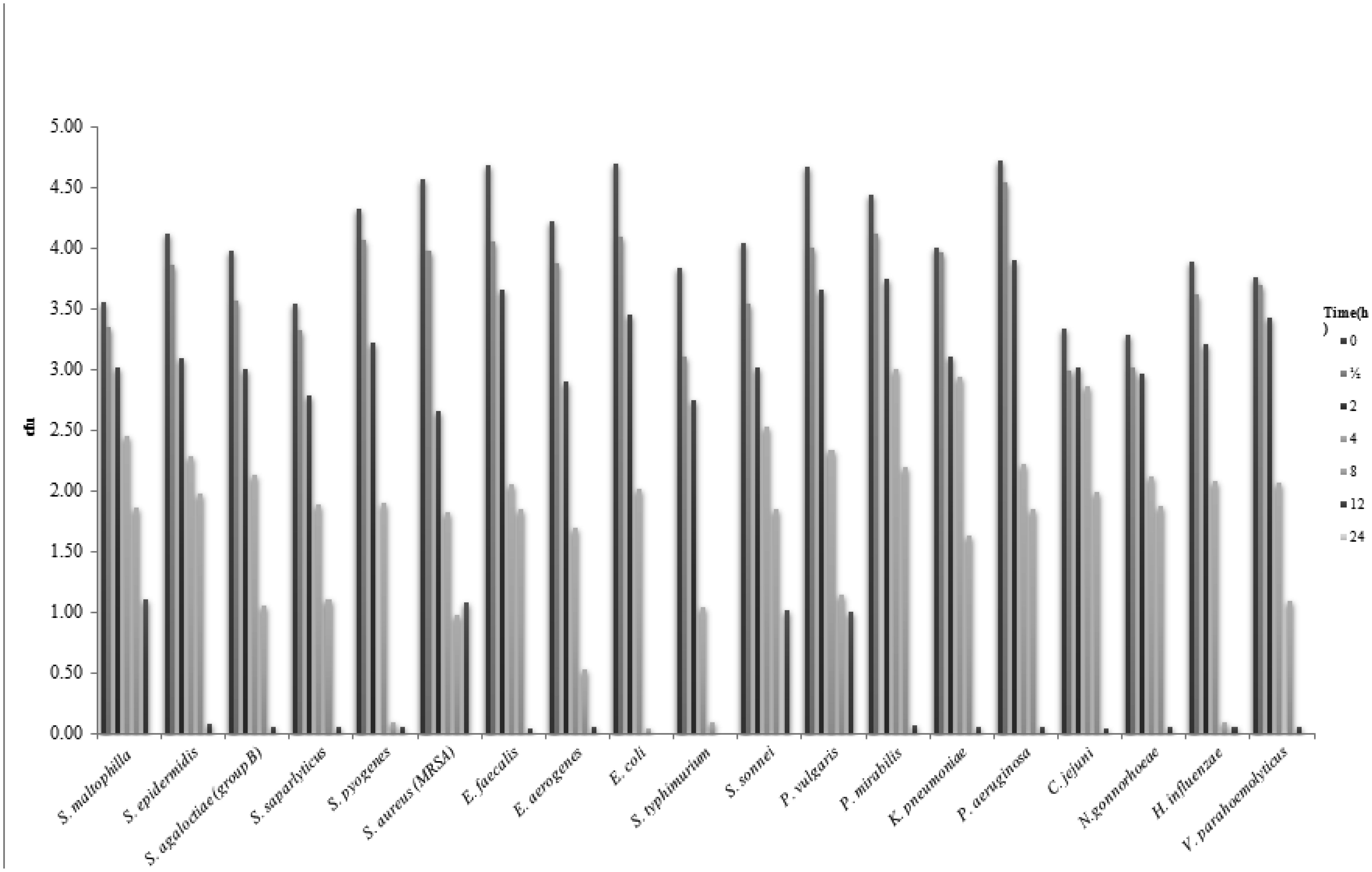
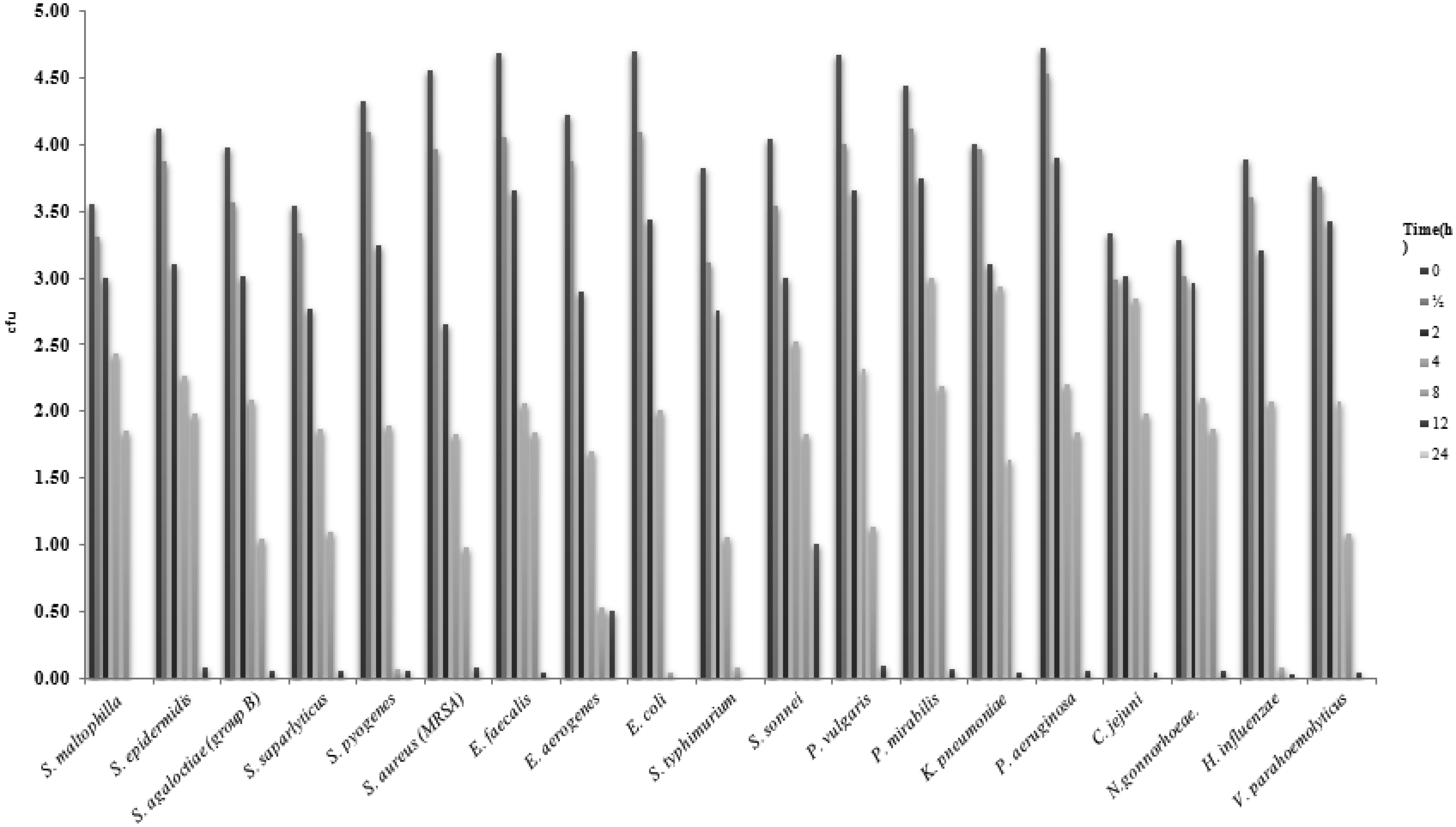
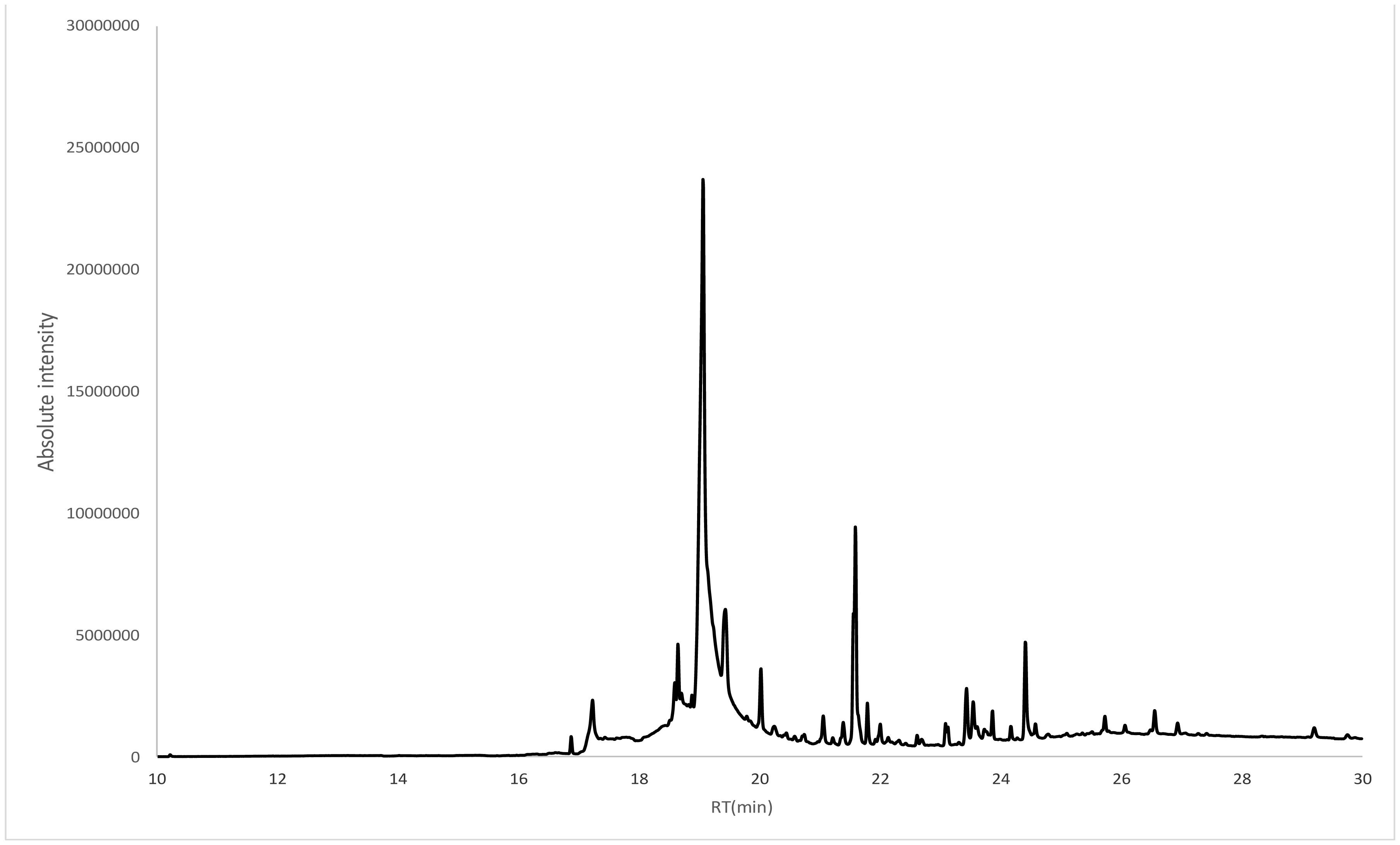
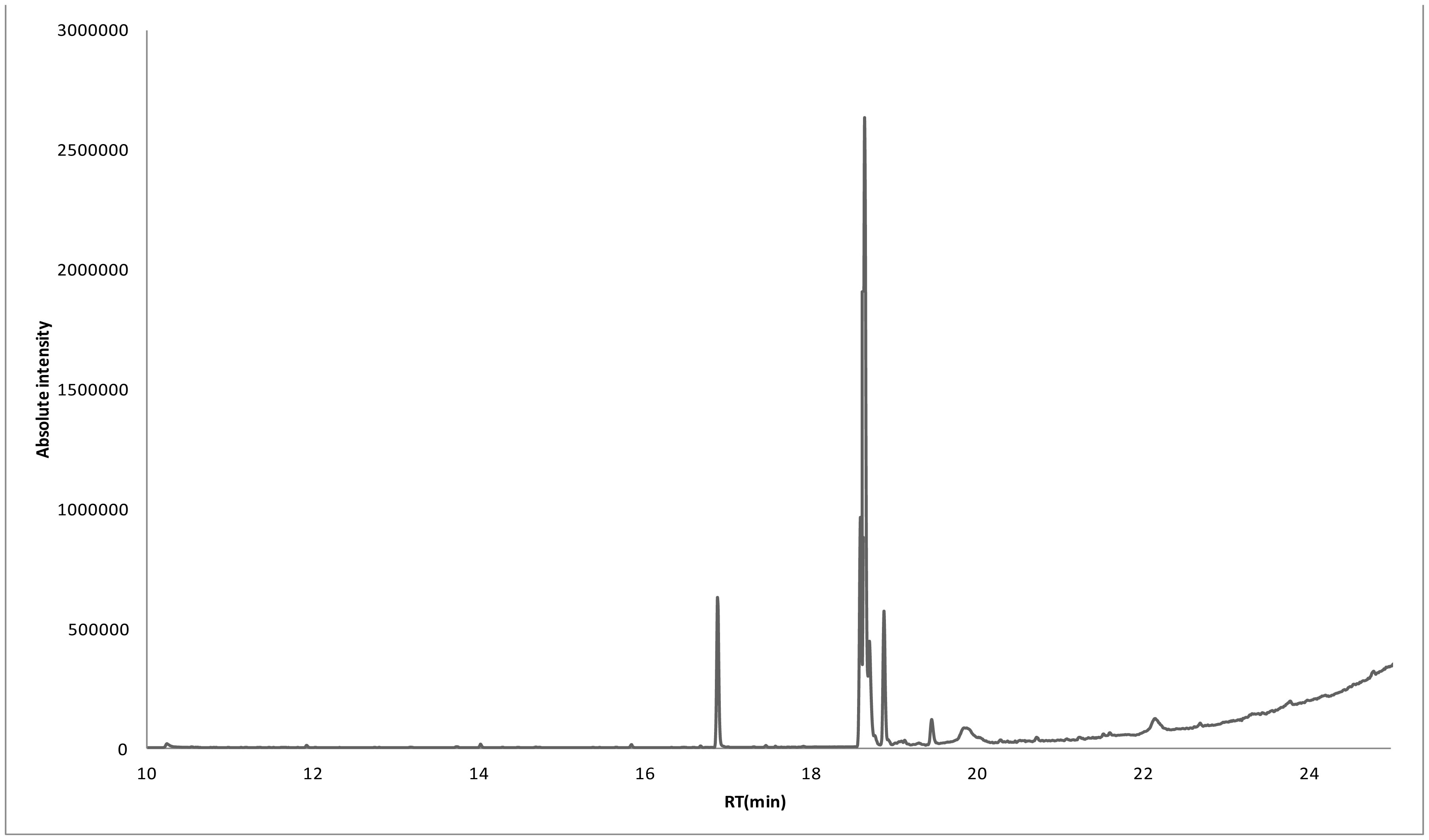
Despite the harsh conditions and limited water resources of the Arabian Peninsula, plants that live in this environment contain a variety of bioactive compounds and have been used in traditional medicines for thousands of years. We investigated the effects of ethanol extracts of Tamarix arabica and Salvadora persica on Gram-negative and Gram-positive bacteria. The investigations were include; the inhibition of the bacterial growth, determination of MIC and MBC, detection of kill-time, potassium and phosphorus leakages and detection of the bioactive compounds by the GC-MS analysis. The tested extracts in combination, at a 1:1 volume ratio, showed high inhibitory effects, as reflected by the minimum inhibitory concentrations and minimum bactericidal concentrations. The new EC plate was used to determined MBC and kill-time. Further, the detection of phosphate and potassium leakage indicated a loss of selective permeability of the cytoplasmic membrane after treatment with these extracts. The bioactive compounds in the ethanol extracts of T. arabica and S. persica may offer a less expensive and natural alternative to pharmaceuticals.
Citation: Awatif A. Al-Judaibi. Tamarix arabica and Salvadora persica as antibacterial agents[J]. AIMS Microbiology, 2020, 6(2): 121-143. doi: 10.3934/microbiol.2020008
Despite the harsh conditions and limited water resources of the Arabian Peninsula, plants that live in this environment contain a variety of bioactive compounds and have been used in traditional medicines for thousands of years. We investigated the effects of ethanol extracts of Tamarix arabica and Salvadora persica on Gram-negative and Gram-positive bacteria. The investigations were include; the inhibition of the bacterial growth, determination of MIC and MBC, detection of kill-time, potassium and phosphorus leakages and detection of the bioactive compounds by the GC-MS analysis. The tested extracts in combination, at a 1:1 volume ratio, showed high inhibitory effects, as reflected by the minimum inhibitory concentrations and minimum bactericidal concentrations. The new EC plate was used to determined MBC and kill-time. Further, the detection of phosphate and potassium leakage indicated a loss of selective permeability of the cytoplasmic membrane after treatment with these extracts. The bioactive compounds in the ethanol extracts of T. arabica and S. persica may offer a less expensive and natural alternative to pharmaceuticals.

| [1] |
Bueno I, Williams-Nguyen J, Hwang H, et al. (2018) Systematic review: impact of point sources on antibiotic-resistant bacteria in the natural environment. Zoonoses Public Health 65: e162-e184. doi: 10.1111/zph.12426

|
| [2] |
Berendonk TU, Manaia CM, Merlin C, et al. (2015) Tackling antibiotic resistance: the environmental framework. Nat Rev Microbiol 13: 310. doi: 10.1038/nrmicro3439
|
| [3] |
Baquero F, Martínez JL, Cantón R (2008) Antibiotics and antibiotic resistance in water environments. Curr Opin Biotechnol 19: 260-265. doi: 10.1016/j.copbio.2008.05.006
|
| [4] |
Zhang QQ, Ying GG, Pan CG, et al. (2015) Comprehensive evaluation of antibiotics emission and fate in the river basins of China: source analysis, multimedia modeling, and linkage to bacterial resistance. Environ Sci Technol 49: 6772-6782. doi: 10.1021/acs.est.5b00729
|
| [5] |
Schwartz T, Kohnen W, Jansen B, et al. (2003) Detection of antibiotic-resistant bacteria and their resistance genes in wastewater, surface water, and drinking water biofilms. FEMS Microbiol Ecol 43: 325-335. doi: 10.1111/j.1574-6941.2003.tb01073.x
|
| [6] |
Hocquet D, Muller A, Bertrand X (2016) What happens in hospitals does not stay in hospitals: antibiotic-resistant bacteria in hospital wastewater systems. J Hosp Infect 93: 395-402. doi: 10.1016/j.jhin.2016.01.010
|
| [7] |
Qiao M, Ying GG, Singer AC, et al. (2018) Review of antibiotic resistance in China and its environment. Environ Int 110: 160-172. doi: 10.1016/j.envint.2017.10.016
|
| [8] | Al-Snafi AE (2018) Arabian medicinal plants for the treatment of intestinal disorders-plant based review (part 1). IOSR J Pharm 8: 53-66. |
| [9] |
Prabhakar J, Senthilkumar M, Priya MS, et al. (2010) Evaluation of antimicrobial efficacy of herbal alternatives (Triphala and green tea polyphenols), MTAD, and 5% sodium hypochlorite against Enterococcus faecalis biofilm formed on tooth substrate: an in vitro study. J Endod 36: 83-86. doi: 10.1016/j.joen.2009.09.040
|
| [10] | Angaji EBSA, Angaji SM (2009) Antimicrobial effects of four medicinal plants on dental plaque. J Med Plants Res 3: 132-137. |
| [11] |
Stanković N, Mihajilov-Krstev T, Zlatković B, et al. (2016) Antibacterial and antioxidant activity of traditional medicinal plants from the Balkan Peninsula. NJAS-Wageningen J Life Sci 78: 21-28. doi: 10.1016/j.njas.2015.12.006
|
| [12] |
Marasini BP, Baral P, Aryal P, et al. (2015) Evaluation of antibacterial activity of some traditionally used medicinal plants against human pathogenic bacteria. BioMed Res Int 2015: 265425. doi: 10.1155/2015/265425
|
| [13] |
Elisha IL, Botha FS, McGaw LJ, et al. (2017) The antibacterial activity of extracts of nine plant species with good activity against Escherichia coli against five other bacteria and cytotoxicity of extracts. BMC Complementary Atern Med 17: 133. doi: 10.1186/s12906-017-1645-z
|
| [14] |
Khan A, Mehmood S, Ahmad I, et al. (2017) Antimicrobial and phytotoxic activities of new important xeric plants. Pak J Phytopathol 29: 29-39. doi: 10.33866/phytopathol.029.01.0319
|
| [15] |
Hosseinzadeh S, Jafarikukhdan A, Hosseini A, et al. (2015) The application of medicinal plants in traditional and modern medicine: a review of Thymus vulgaris. Int J Clin Med 6: 635-642. doi: 10.4236/ijcm.2015.69084
|
| [16] | Mittal S, Nautiyal U (2019) A review: herbal remedies used for the treatment of mouth ulcer. Int J Health Clin Res 2: 17-23. |
| [17] |
Brum A, Pereira SA, Owatari MS, et al. (2017) Effect of dietary essential oils of clove basil and ginger on Nile tilapia (Oreochromis niloticus) following challenge with Streptococcus agalactiae. Aquaculture 468: 235-243. doi: 10.1016/j.aquaculture.2016.10.020
|
| [18] | Ali M, Alhazmi HA, Ansari SH, et al. (2019) Tamarix aphylla (L.) karst. phytochemical and bioactive profile compilations of less discussed but effective naturally growing Saudi plant. Plant Human Health 3: 343-352. |
| [19] |
Langmead L, Rampton DS (2001) Herbal treatment in gastrointestinal and liver disease—benefits and dangers. Aliment Pharmacol Ther 15: 1239-1252. doi: 10.1046/j.1365-2036.2001.01053.x
|
| [20] |
Okawa Y, Fukudo S, Sanada H (2019) Specific foods can reduce symptoms of irritable bowel syndrome and functional constipation: a review. BioPsychoSoc Med 13: 10. doi: 10.1186/s13030-019-0152-5
|
| [21] |
Kouidhi B, Al Qurashi YMA, Chaieb K (2015) Drug resistance of bacterial dental biofilm and the potential use of natural compounds as alternative for prevention and treatment. Microb pathog 80: 39-49. doi: 10.1016/j.micpath.2015.02.007
|
| [22] |
Saleh MY, Chaturvedi S, Ibrahim B, et al. (2019) Hearbal detox extract formulation from seven wonderful natural herbs: Garlic, Ginger, Honey, Carrots, Aloe Vera, Dates, & Corn. Asian J Pharm Res Dev 7: 22-30. doi: 10.22270/ajprd.v7i3.485
|
| [23] | El-Shabasy A (2016) Survey on medicinal plants in the flora of Jizan region, Saudi Arabia. Int J Bot Stud 2: 38-59. |
| [24] | Hamza N, Berke B, Umar A, et al. (2019) A review of Algerian medicinal plants used in the treatment of diabetes. J Ethnopharmacol 111841. |
| [25] |
Manoj G, Sasmal D, Nagori BP (2011) Salvadora persica (Meswak): chewing stick for complete oral care. Int J Pharmacol 7: 440-445. doi: 10.3923/ijp.2011.440.445
|
| [26] |
Alnuqaydan AM, Rah B (2019) Tamarix articulata (T. articulata)-an important halophytic medicinal plant with potential pharmacological properties. Curr Pharm Biotechnol 20: 285-292. doi: 10.2174/1389201020666190318120103
|
| [27] | Clinical and Laboratory Standards Institute (CLSI) (2007) Performance standards for antimicrobial susceptibility testing; seventeenth information supplement.27. |
| [28] |
Krishnan M, Dey DK, Sharma C, et al. (2019) Antibacterial activity of Weissella confusa by disc diffusion method. Bangladesh J Pharmacol 14. doi: 10.3329/bjp.v14i3.41545
|
| [29] |
Wiegand I, Hilpert K, Hancock REW (2008) Agar and broth dilution methods to determine the minimal inhibitory concentration (MIC) of antimicrobial substances. Nat Protoc 3: 163-175. doi: 10.1038/nprot.2007.521
|
| [30] |
Biswas K, Upadhayay S, Rapsang GF, et al. (2017) Antibacterial and synergistic activity against b-Lactamase-Producing nosocomial bacteria by bacteriocin of LAB Isolated from lesser known traditionally fermented products of India. HAYATI J Biosci 24: 87-95. doi: 10.1016/j.hjb.2017.08.008
|
| [31] |
Lambert RJW, Skandamis PN, Coote PJ, et al. (2001) A study of the minimum inhibitory concentration and mode of action of oregano essential oil, thymol and carvacrol. J Appl Microbiol 91: 453-462. doi: 10.1046/j.1365-2672.2001.01428.x
|
| [32] | Madigan MT, Versalovic J, Carroll KC, et al. (2011) Manual of clinical microbiology ASM Press, 1169-1170. |
| [33] |
Hernandes C, Coppede JDS, Bertoni BWR, et al. (2013) Flash microbiocide: A rapid and economic method for determination of MBC and MFC. Am J Plant Sci 4: 850-852. doi: 10.4236/ajps.2013.44104
|
| [34] |
Shami AY, Almasri RA (2018) Research article bacteriostatic and bactericidal activity of deer musk on multidrug resistance bacteria. Pak J Biol Sci 21: 331-339. doi: 10.3923/pjbs.2018.331.339
|
| [35] |
Plata KB, Riosa S, Singh CR, et al. (2013) Targeting of PBP1 by B-lactams determines recA/SOS response activation in heterogeneous MRSA clinical strains. Plos One 8: e61083. doi: 10.1371/journal.pone.0061083
|
| [36] | Kbajpai V, Sharma A, Baek KH (2014) Antibacterial mode of action of the essential oil obtained from Chamaecyparis obtusa sawdust on the membrane integrity of selected foodborne pathogens. Food Technol Biotechnol 52: 109-118. |
| [37] | Al-Judaibi A (2014) Antibacterial effects of extracts of two types of Red Sea Algae. J Biosci Med 2: 74-82. |
| [38] |
Andrews JM (2001) Determination of minimum inhibitory concentrations. J Antimicrob Chemother 49: 1049-1049. doi: 10.1093/jac/dkf083
|
| [39] |
Chikezie IO (2017) Determination of Minimum Inhibitory Concentration (MIC) and Minimum Bactericidal Concentration (MBC) using a novel dilution tube method. Afr J Microbiol Res 11: 977-980. doi: 10.5897/AJMR2017.8545
|
| [40] |
Forney CF, Sharon JP (2016) Chilling-induced potassium leakage of cultured cells. Physiologia Plantarum 78: 193-196. doi: 10.1111/j.1399-3054.1990.tb02080.x
|
| [41] |
Johnston MD, Hanlon GW, Denyer SP, et al. (2003) Membrane damage to bacteria caused by single and combined biocides. J Appl Microbiol 94: 1015-1023. doi: 10.1046/j.1365-2672.2003.01923.x
|
| [42] |
Sundar RDV, Srikanth L, Manognya PS, et al. (2019) In vitro antibacterial activity of Dracaena victoria leaf extract. Bangladesh J Pharmacol 14: 202-203. doi: 10.3329/bjp.v14i4.43807
|
| [43] |
Kovalskaya NY, Herndon EE, Foster-Frey JA, et al. (2019) Antimicrobial activity of bacteriophage derived triple fusion protein against Staphylococcus aureus. AIMS Microbiol 5: 158. doi: 10.3934/microbiol.2019.2.158
|
| [44] |
Kanthal LK, Dey A, Satyavathi K, et al. (2014) GC-MS analysis of bio-active compounds in methanolic extract of Lactuca runcinata DC. Pharmacogn Res 6: 58. doi: 10.4103/0974-8490.122919
|
| [45] | Asha KR, Priyanga S, Hemmalakshmi S, et al. (2017) GC-MS Analysis of the Ethanolic Extract of the whole Plant Drosera indica L. J Pharmacogn Phytochem Res 9: 685-688. |
| [46] | Azwanida NN (2015) A review on the extraction methods use in medicinal plants, principle, strength and limitation. Med Aromat Plants 4: 2167-0412. |
Figures(6) / Tables(8)

Awatif A. Al-Judaibi. Tamarix arabica and Salvadora persica as antibacterial agents[J]. AIMS Microbiology, 2020, 6(2): 121-143. doi: 10.3934/microbiol.2020008


 DownLoad: