Theoretical evaluation of the power efficiency of a moored hybrid floating platform for wind and wave energy production in the Greek seas

Kimon Kardakaris; Dimitrios N Konispoliatis; Takvor H Soukissian; Kimon Kardakaris; Dimitrios N Konispoliatis; Takvor H Soukissian

doi:10.3934/geosci.2023009

AIMS Geosciences

2023, Volume 9, Issue 1: 153-183. doi: 10.3934/geosci.2023009

Previous Article Next Article

Research article Special Issues

Theoretical evaluation of the power efficiency of a moored hybrid floating platform for wind and wave energy production in the Greek seas

1.
Laboratory for Floating Structures and Mooring Systems, Division of Marine Structures, School of Naval Architecture and Marine Engineering, National Technical University of Athens, 9 Heroon Polytechniou Avenue, GR 157–73 Athens, Greece
2.
Institute of Oceanography, Hellenic Centre for Marine Research, 190 13 Anavyssos, Greece

Received: 27 November 2022 Revised: 24 January 2023 Accepted: 07 February 2023 Published: 22 February 2023

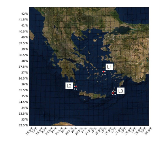
In this study, an extreme value analysis of wind and wave parameters is presented for three specific locations in the Greek seas that are known to be advantageous in terms of joint power production (both offshore wind and wave) and bathymetric conditions. The analysis is conducted via the Peak-Over-Threshold method, examining wind speed, significant wave height and peak wave period data from the ERA5 reanalysis dataset. Moreover, a multi-purpose floating platform suitable for offshore energy production is presented, which combines wind and wave energy resources exploitation and can be adequately utilized at the selected locations. The analysis is built to incorporate the solutions of the diffraction, motion-dependent and pressure-dependent radiation problems around the floating structure, along with the mooring line and wind turbine (WT) characteristics. Subsequently, a coupled hydro-aero-elastic analysis was performed in the frequency domain, while a dynamic analysis was conducted in order to evaluate the mooring characteristics. Lastly, offshore wind output and absorbed wave energy values were estimated, and different types of mooring systems were compared in terms of efficiency. It has been concluded that the wind energy capacity factor is higher than 50% in all the examined locations, and by the mooring system comparison, the tension-leg platform (TLP) represents the best-case scenario for wave energy absorption.
- multi-purpose floating platform,
- catenary mooring line system,
- hybrid wind-wave energy,
- extreme value analysis,
- Greek seas
Citation: Kimon Kardakaris, Dimitrios N Konispoliatis, Takvor H Soukissian. Theoretical evaluation of the power efficiency of a moored hybrid floating platform for wind and wave energy production in the Greek seas[J]. AIMS Geosciences, 2023, 9(1): 153-183. doi: 10.3934/geosci.2023009

Related Papers:

Abstract

In this study, an extreme value analysis of wind and wave parameters is presented for three specific locations in the Greek seas that are known to be advantageous in terms of joint power production (both offshore wind and wave) and bathymetric conditions. The analysis is conducted via the Peak-Over-Threshold method, examining wind speed, significant wave height and peak wave period data from the ERA5 reanalysis dataset. Moreover, a multi-purpose floating platform suitable for offshore energy production is presented, which combines wind and wave energy resources exploitation and can be adequately utilized at the selected locations. The analysis is built to incorporate the solutions of the diffraction, motion-dependent and pressure-dependent radiation problems around the floating structure, along with the mooring line and wind turbine (WT) characteristics. Subsequently, a coupled hydro-aero-elastic analysis was performed in the frequency domain, while a dynamic analysis was conducted in order to evaluate the mooring characteristics. Lastly, offshore wind output and absorbed wave energy values were estimated, and different types of mooring systems were compared in terms of efficiency. It has been concluded that the wind energy capacity factor is higher than 50% in all the examined locations, and by the mooring system comparison, the tension-leg platform (TLP) represents the best-case scenario for wave energy absorption.

References

[1]	GWEC (2021) Global offshore wind report. Available from: https://gwec.net/global-offshore-wind-report-2021/.
[2]	Butterfield S, Musial W, Jonkman J, et al. (2007) Engineering challenges for floating offshore wind turbines. National Renewable Energy Laboratory, Golden, United States. Available from: https://www.nrel.gov/docs/fy07osti/38776.pdf.
[3]	Huijs F, de Ridder EJ, Savenije F (2014) Comparison of model tests and coupled simulations for a semi-submersible floating wind turbine. Int Conf Offshore Mech Arct Eng 45530: V09AT09A012. https://doi.org/10.1115/OMAE2014-23217
[4]	Roddier D, Cermelli C, Aubault A, et al. (2010) Windfloat: A floating foundation for offshore wind turbines. J Renewable Sustainable Energy 2: 033104. https://doi.org/10.1063/1.3435339 doi: 10.1063/1.3435339
[5]	Borg M, Walkusch Jensen M, Urquhart S, et al. (2020) Technical definition of the tetraspar demonstrator floating wind turbine foundation. Energies 13: 4911. https://doi.org/10.3390/en13184911 doi: 10.3390/en13184911
[6]	Galvan J, Sánchez-Lara MJ, Mendikoa I, et al. (2018) NAUTILUS-DTU10 MW Floating Offshore Wind Turbine at Gulf of Maine: Public numerical models of an actively ballasted semisubmersible. J Phy Conf Ser 1102: 012015. https://doi.org/10.1088/1742-6596/1102/1/012015 doi: 10.1088/1742-6596/1102/1/012015
[7]	Robertson A, Jonkman J, Masciola M, et al. (2014) Definition of the semisubmersible floating system for phase Ⅱ of OC4. National Renewable Energy Laboratory, Golden, United States. Available from: https://www.nrel.gov/docs/fy14osti/60601.pdf.
[8]	Robertson AN, Wendt F, Jonkman JM, et al. (2017) OC5 project phase Ⅱ: validation of global loads of the deepcwind floating semisubmersible wind turbine. Energy Procedia 137: 38–57. https://doi.org/10.1016/j.egypro.2017.10.333 doi: 10.1016/j.egypro.2017.10.333
[9]	Uzunoglu E, Karmakar D, Guedes Soares C (2016) Floating offshore wind platforms, Floating offshore wind farms, Springer, 53–76. https://doi.org/10.1007/978-3-319-27972-5_4
[10]	Pelagic Power AS (2010) Mobilising the total offshore renewable energy resource. Available from: www.pelagicpower.no.
[11]	Marine Power Systems. Available from: https://www.marinepowersystems.co.uk/dualsub/.
[12]	Floating Power Plant (FPP). Available from: http://www.floatingpowerplant.com/.
[13]	Bachynski EE, Moan T (2013) Point absorber design for a combined wind and wave energy converter on a tension-leg support structure. Int Conf Offshore Mech Arct Eng 55423: V008T09A025. https://doi.org/10.1115/OMAE2013-10429
[14]	Muliawan MJ, Karimirad M, Gao Z, et al. (2013) Extreme responses of a combined spar-type floating wind turbine and floating wave energy converter (STC) system with survival modes. Ocean Eng 65: 71–82. https://doi.org/10.1016/j.oceaneng.2013.03.002
[15]	Muliawan MJ, Karimirad M, Moan T (2013) Dynamic response and power performance of a combined spar-type floating wind turbine and coaxial floating wave energy converter. Renewable Energy 50: 47–57. https://doi.org/10.1016/j.renene.2012.05.025 doi: 10.1016/j.renene.2012.05.025
[16]	Veigas M, Iglesias G (2015) A hybrid wave-wind offshore farm for an island. International J Green Energy 12: 570–576. https://doi.org/10.1080/15435075.2013.871724 doi: 10.1080/15435075.2013.871724
[17]	Michailides C, Gao Z, Moan T (2016) Experimental and numerical study of the response of the offshore combined wind/wave energy concept SFC in extreme environmental conditions. Mar Struct 50: 35–54. https://doi.org/10.1016/j.marstruc.2016.06.005 doi: 10.1016/j.marstruc.2016.06.005
[18]	Michailides C, Gao Z, Moan T (2016) Experimental study of the functionality of a semisubmersible wind turbine combined with flap-type Wave Energy Converters. Renewable Energy 93: 675–690. https://doi.org/10.1016/j.renene.2016.03.024 doi: 10.1016/j.renene.2016.03.024
[19]	Gao Z, Moan T, Wan L, et al. (2016) Comparative numerical and experimental study of two combined wind and wave energy concepts. J Ocean Eng Sci 1: 36–51. https://doi.org/10.1016/j.joes.2015.12.006 doi: 10.1016/j.joes.2015.12.006
[20]	Karimirad M, Koushan K (2016) WindWEC: Combining wind and wave energy inspired by hywind and wavestar. 2016 IEEE Int Conf Renewable Energy Res Appl, 96–101. https://doi.org/10.1109/ICRERA.2016.7884433
[21]	Wang Y, Zhang L, Michailides C, et al. (2020) Hydrodynamic Response of a Combined Wind-Wave Marine Energy Structure. J Mar Sci Eng 8: 253. https://doi.org/10.3390/jmse8040253 doi: 10.3390/jmse8040253
[22]	Wang B, Deng Z, Zhang B (2022) Simulation of a novel wind–wave hybrid power generation system with hydraulic transmission. Energy 238: 121833. https://doi.org/10.1016/j.energy.2021.121833 doi: 10.1016/j.energy.2021.121833
[23]	Aubault A, Alves M, Sarmento A, et al. (2011) Modeling of an oscillating water column on the floating foundation WINDFLOAT. Int Conf Ocean Offshore Arct Eng, 235–246. https://doi.org/10.1115/OMAE2011-49014
[24]	Mazarakos T, Konispoliatis D, Manolas D, et al. (2015) Modelling of an offshore multi-purpose floating structure supporting a wind turbine including second-order wave loads. 11th Eur Wave Tidal Energy Conf, 7–10.
[25]	Mazarakos T, Konispoliatis D, Katsaounis G, et al. (2019) Numerical and experimental studies of a multi-purpose floating TLP structure for combined wind and wave energy exploitation. Mediterr Mar Sci 20: 745–763. https://doi.org/10.12681/mms.19366 doi: 10.12681/mms.19366
[26]	Perez-Collazo C, Greaves D, Iglesias G (2018) A novel hybrid wind-wave energy converter for jacket-frame substructures. Energies 11: 637. https://doi.org/10.3390/en11030637 doi: 10.3390/en11030637
[27]	Perez-Collazo C, Pemberton R, Greaves D, et al. (2019) Monopile-mounted wave energy converter for a hybrid wind-wave system. Energy Conversion and Management 199: 111971. https://doi.org/10.1016/j.enconman.2019.111971 doi: 10.1016/j.enconman.2019.111971
[28]	Sarmiento J, Iturrioz A, Ayllón V, et al. (2019) Experimental modelling of a multi-use floating platform for wave and wind energy harvesting. Ocean Eng 173: 761–773. https://doi.org/10.1016/j.oceaneng.2018.12.046 doi: 10.1016/j.oceaneng.2018.12.046
[29]	Michele S, Renzi E, Perez-Collazo C, et al. (2019) Power extraction in regular and random waves from an OWC in hybrid wind-wave energy systems. Ocean Eng 191: 106519. https://doi.org/10.1016/j.oceaneng.2019.106519 doi: 10.1016/j.oceaneng.2019.106519
[30]	Zhou Y, Ning D, Shi W, et al. (2020) Hydrodynamic investigation on an OWC wave energy converter integrated into an offshore wind turbine monopile. Coast Eng 162: 103731. https://doi.org/10.1016/j.coastaleng.2020.103731 doi: 10.1016/j.coastaleng.2020.103731
[31]	Konispoliatis DN, Katsaounis GM, Manolas DI, et al. (2021) REFOS: A Renewable Energy Multi-Purpose Floating Offshore System. Energies 14: 3126. https://doi.org/10.3390/en14113126 doi: 10.3390/en14113126
[32]	Konispoliatis D, Mazarakos T, Soukissian T, et al. (2018) REFOS: A multi-purpose floating platform suitable for wind and wave energy exploitation. Proc 11th Int Conf Deregulated Electr Mark Issues South East Eur, 20–21.
[33]	Konispoliatis DN, Manolas DI, Voutsinas SG, et al. (2022) Coupled Dynamic Response of an Offshore Multi-Purpose Floating Structure Suitable for Wind and Wave Energy Exploitation. Front Energy Res 10: 920151.
[34]	Esteban MD, Diez JJ, López JS, et al. (2011) Why offshore wind energy? Renewable Energy 36: 444–450. https://doi.org/10.1016/j.renene.2010.07.009 doi: 10.1016/j.renene.2010.07.009
[35]	Martinez A, Iglesias G (2021) Multi-parameter analysis and mapping of the levelised cost of energy from floating offshore wind in the Mediterranean Sea. Energy Convers Manage 243: 114416. https://doi.org/10.1016/j.enconman.2021.114416 doi: 10.1016/j.enconman.2021.114416
[36]	Soukissian T, Papadopoulos A, Skrimizeas P, et al. (2017) Assessment of offshore wind power potential in the Aegean and Ionian Seas based on high-resolution hindcast model results. AIMS Energy 5: 268–289. https://doi.org/10.3934/energy.2017.2.268 doi: 10.3934/energy.2017.2.268
[37]	Kardakaris K, Boufidi I, Soukissian T (2021) Offshore wind and wave energy complementarity in the Greek seas based on ERA5 data. Atmosphere 12: 1360. https://doi.org/10.3390/atmos12101360 doi: 10.3390/atmos12101360
[38]	EMODnet Bathymetry. Available from: https://portal.emodnet-bathymetry.eu/.
[39]	Hersbach H, Bell B, Berrisford P, et al. (2020) The ERA5 global reanalysis. QJR Meteorol Soc 146: 1999–2049. https://doi.org/10.1002/qj.3803 doi: 10.1002/qj.3803
[40]	Farjami H, Hesari ARE (2020) Assessment of sea surface wind field pattern over the Caspian Sea using EOF analysis. Reg Stud Mar Sci 35: 101254. https://doi.org/10.1016/j.rsma.2020.101254 doi: 10.1016/j.rsma.2020.101254
[41]	de Assis Tavares LF, Shadman M, de Freitas Assad LP, et al. (2020) Assessment of the offshore wind technical potential for the Brazilian Southeast and South regions. Energy 196: 117097. https://doi.org/10.1016/j.energy.2020.117097 doi: 10.1016/j.energy.2020.117097
[42]	Bruno MF, Molfetta MG, Totaro V, et al. (2020) Performance assessment of ERA5 wave data in a swell dominated region. J Mar Sci Eng 8: 214. https://doi.org/10.3390/jmse8030214 doi: 10.3390/jmse8030214
[43]	Karathanasi FE, Soukissian TH, Hayes DR (2022) Wave Analysis for Offshore Aquaculture Projects: A Case Study for the Eastern Mediterranean Sea. Climate 10: 2 https://doi.org/10.3390/cli10010002 doi: 10.3390/cli10010002
[44]	Soukissian TH, Tsalis C (2015) The effect of the generalized extreme value distribution parameter estimation methods in extreme wind speed prediction. Nat Hazards 78: 1777–1809. https://doi.org/10.1007/s11069-015-1800-0 doi: 10.1007/s11069-015-1800-0
[45]	Soukissian TH, Tsalis C (2018) Effects of parameter estimation method and sample size in metocean design conditions. Ocean Eng 169: 19–37. https://doi.org/10.1016/j.oceaneng.2018.09.017 doi: 10.1016/j.oceaneng.2018.09.017
[46]	Soukissian TH, Kalantzi GD (2006) Extreme value analysis methods used for extreme wave prediction. Sixteenth Int Offshore Polar Eng Conf. OnePetro.
[47]	Sartini L, Mentaschi L, Besio G (2015) Comparing different extreme wave analysis models for wave climate assessment along the Italian coast. Coastal Eng 100: 37–47. https://doi.org/10.1016/j.coastaleng.2015.03.006 doi: 10.1016/j.coastaleng.2015.03.006
[48]	Park SB, Shin SY, Jung KH, et al. (2020) Extreme Value Analysis of Metocean Data for Barents Sea. J Ocean Eng Technol 34: 26–36. https://doi.org/10.26748/KSOE.2019.094 doi: 10.26748/KSOE.2019.094
[49]	Devis-Morales A, Montoya-Sánchez RA, Bernal G, et al. (2017) Assessment of extreme wind and waves in the Colombian Caribbean Sea for offshore applications. Appl Ocean Res 69: 10–26. https://doi.org/10.1016/j.apor.2017.09.012 doi: 10.1016/j.apor.2017.09.012
[50]	Ferreira JA, Guedes Soares C (1998) An application of the peaks over threshold method to predict extremes of significant wave height. J Offshore Mech Arct Eng 120: 165–176. https://doi.org/10.1115/1.2829537 doi: 10.1115/1.2829537
[51]	Caires S, Sterl A (2005) 100-year return value estimates for ocean wind speed and significant wave height from the ERA-40 data. J Clim 18: 1032–1048. https://doi.org/10.1175/JCLI-3312.1 doi: 10.1175/JCLI-3312.1
[52]	Méndez FJ, Menéndez M, Luceño A, et al. (2006) Estimation of the long‐term variability of extreme significant wave height using a time‐dependent peak over threshold (pot) model. J Geophys Res Oceans 111.
[53]	Dissanayake P, Flock T, Meier J, et al. (2021) Modelling short-and long-term dependencies of clustered high-threshold exceedances in significant wave heights. Mathematics 9: 2817. https://doi.org/10.3390/math9212817 doi: 10.3390/math9212817
[54]	Coles S (2001) An Introduction to Statistical Modeling of Extreme Values. Bristol, UK. Springer.
[55]	Lemos IP, Lima AMG, Duarte MAV (2020) thresholdmodeling: A Python package for modeling excesses over a threshold using the Peak-Over-Threshold Method and the Generalized Pareto Distribution. J Open Source Software 5: 2013. https://doi.org/10.21105/joss.02013 doi: 10.21105/joss.02013
[56]	Bak C, Zahle F, Bitsche R, et. al. (2013) The DTU 10-MW reference wind turbine. Dan Wind Power Res 2013.
[57]	Konispoliatis D, Mazarakos T, Mavrakos S (2016) Hydrodynamic analysis of three-unit arrays of floating annular oscillating-water column wave energy converters. Appl Ocean Res 61: 42–64. https://doi.org/10.1016/j.apor.2016.10.003 doi: 10.1016/j.apor.2016.10.003
[58]	Mavrakos SA, Koumoutsakos P (1987) Hydrodynamic interaction among vertical axisymmetric bodies restrained in waves. Appl Ocean Res 9: 128–140. https://doi.org/10.1016/0141-1187(87)90017-4 doi: 10.1016/0141-1187(87)90017-4
[59]	Mavrakos S (1991) Hydrodynamic coefficients for groups of interacting vertical axisymmetric bodies. Ocean Eng 18: 485–515. https://doi.org/10.1016/0029-8018(91)90027-N doi: 10.1016/0029-8018(91)90027-N
[60]	Konispoliatis D, Mazarakos T, Katsidoniotaki E, et al. (2019) Efficiency of an array of OWC devices equipped with air turbines with pitch control. Proc 13th Eur Wave Tidal Energy Conf, Napoli, Italy, 1–6.
[61]	Falnes J (2002) Ocean Waves and Oscillating Systems. Cambridge University Press: Cambridge, UK; New York, NY, USA.
[62]	Anchor Marine & Industrial Supply Inc. Available from: https://anchormarinehouston.com/chain/
[63]	Mavrakos S (1995) User's Manual for the Software HAMVAB. School of Naval Architecture and Marine Engineering, Laboratory for Floating Structures and Mooring Systems, Athens, Greece.
[64]	Mavrakos SA, McIver P (1997) Comparison of methods for computing hydrodynamic characteristics of arrays of wave power devices. Appl Ocean Res 19: 283–291. https://doi.org/10.1016/S0141-1187(97)00029-1 doi: 10.1016/S0141-1187(97)00029-1
[65]	Konispoliatis DN, Mavrakos SA (2016) Hydrodynamic analysis of an array of interacting free-floating oscillating water column (OWC's) devices. Ocean Eng 111: 179–197. https://doi.org/10.1016/j.oceaneng.2015.10.034 Get righ doi: 10.1016/j.oceaneng.2015.10.034Getrigh
[66]	Konispoliatis DN, Chatjigeorgiou IK, Mavrakos SA (2022) Hydrodynamics of a Moored Permeable Vertical Cylindrical Body. J Mar Sci Eng 10: 403. https://doi.org/10.3390/jmse10030403 doi: 10.3390/jmse10030403
[67]	NREL DTU 10 MW. Available from: https://nrel.github.io/turbine-models/DTU_10MW_178_RWT_v1.html.
[68]	Evans D V (1978) The oscillating water column wave-energy device. IMA J Appl Math 22: 423–433.
[69]	Konispoliatis DN, Mavrakos AS, Mavrakos SA (2020) Efficiency of an oscillating water column device for several mooring systems. Developments in Renewable Energies Offshor, CRC Press. 666–673.
[70]	DNV GL Class Guideline: DNVGL-CG-0130. Wave Loads. Available from: https://studylib.net/doc/25365327/dnvgl-cg-0130.
[71]	Duan F, Hu Z, Niedzwecki JM (2016) Model test investigation of a spar floating wind turbine. Mar Struct 49: 76–96. https://doi.org/10.1016/j.marstruc.2016.05.011 doi: 10.1016/j.marstruc.2016.05.011
[72]	Russo S, Contestabile P, Bardazzi A, et al. (2021) Dynamic loads and response of a spar buoy wind turbine with pitch-controlled rotating blades: An experimental study. Energies 14: 3598. https://doi.org/10.3390/en14123598 doi: 10.3390/en14123598
[73]	Life-Cycle Assessment of a Renewable Energy Multi-Purpose Floating Offshore System, REFOS (709526) project. EU Framework Program for Research and Innovation, Research Fund for Coal and Steel. Available from: www.refos-project.eu.

Reader Comments

Your name:*

Email:*
© 2023 the Author(s), licensee AIMS Press. This is an open access article distributed under the terms of the Creative Commons Attribution License (http://creativecommons.org/licenses/by/4.0)