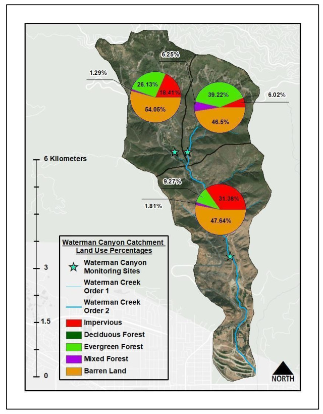
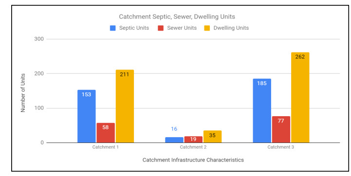
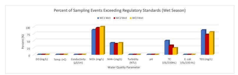
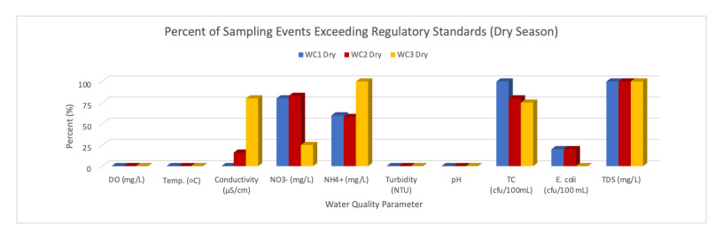
Sources of stream impairments are well known; however, less attention has centered on characterizing the extent to which human-environmental factors influence headwater stream quality within semi-arid watersheds. This study quantified the extent to which seasonal weather patterns and landscape attributes contribute to the physicochemical characteristics of two perennial headwater tributaries and their confluence within the semi-arid mountainous region of the Santa Ana River Basin, California. In situ sampling of stream temperature (℃), stream flow rate (m/s), nitrate (NO3-), ammonium (NH4+), turbidity (NTU), dissolved oxygen (DO), conductivity, pH and lab assessments for. E. coli, total coliform (TC) and total dissolved solids (TDS) occurred during dry and wet season conditions. Across sampling locations, multiple parameters (i.e. NO3-, NH4+, TDS, TC) consistently exceeded regulatory standards simultaneously during both the dry and wet seasons, however, the level of concentrations varied between a tributary catchment landscape with high percentage of impervious surfaces (i.e. roads, buildings) and wastewater infrastructure (i.e septic, sewer) versus one characterized by agricultural activities (i.e. crop, livestock) and barren land. Findings illustrate the need for hydrologically comprehensive strategies (i.e. stream headwaters to river mouth) that are community to agency-driven and that support the expansion of monitoring and shared knowledge to mitigate impairments within headwater streams and downstream. Potential avenues for community collaborations that support sustainable water management strategies are highlighted.
Citation: Jennifer B Alford, Jose A Mora. Factors influencing chronic semi-arid headwater stream impairments: a southern California case study[J]. AIMS Geosciences, 2022, 8(1): 98-126. doi: 10.3934/geosci.2022007
Sources of stream impairments are well known; however, less attention has centered on characterizing the extent to which human-environmental factors influence headwater stream quality within semi-arid watersheds. This study quantified the extent to which seasonal weather patterns and landscape attributes contribute to the physicochemical characteristics of two perennial headwater tributaries and their confluence within the semi-arid mountainous region of the Santa Ana River Basin, California. In situ sampling of stream temperature (℃), stream flow rate (m/s), nitrate (NO3-), ammonium (NH4+), turbidity (NTU), dissolved oxygen (DO), conductivity, pH and lab assessments for. E. coli, total coliform (TC) and total dissolved solids (TDS) occurred during dry and wet season conditions. Across sampling locations, multiple parameters (i.e. NO3-, NH4+, TDS, TC) consistently exceeded regulatory standards simultaneously during both the dry and wet seasons, however, the level of concentrations varied between a tributary catchment landscape with high percentage of impervious surfaces (i.e. roads, buildings) and wastewater infrastructure (i.e septic, sewer) versus one characterized by agricultural activities (i.e. crop, livestock) and barren land. Findings illustrate the need for hydrologically comprehensive strategies (i.e. stream headwaters to river mouth) that are community to agency-driven and that support the expansion of monitoring and shared knowledge to mitigate impairments within headwater streams and downstream. Potential avenues for community collaborations that support sustainable water management strategies are highlighted.

| [1] |
Hosen JD, McDonough OT, Febria CM, et al. (2014) Dissolved Organic Matter Quality and Bioavailability Changes Across an Urbanization Gradient in Headwater Streams. Envirn Sci Technol 48: 7817–7824. https://doi.org/10.1021/es501422z doi: 10.1021/es501422z

|
| [2] |
Mallin MA, Johnson VL, Ensign SH (2009) Comparative Impacts of Stormwater Runoff on Water Quality of an Urban, a Suburban, and a Rural Stream. Environ Monit Assess 159: 475–491. https://doi.org/10.1007/s10661-008-0644-4 doi: 10.1007/s10661-008-0644-4
|
| [3] |
Moore AA, Palmer M (2005) Invertebrate Biodiversity in Agricultural and Urban Headwater Streams: Implications for Conservation and Management. Ecol App 15: 1160–1177. https://doi.org/10.1890/04-1484 doi: 10.1890/04-1484
|
| [4] |
Siziba N, Mwedzi T, Muisa N (2021) Assessment of nutrient enrichment and heavy metal pollution of headwater streams of Bulawayo, Zimbabwe. Phys Chem Earth 122: 102912. https://doi.org/10.1016/j.pce.2020.102912 doi: 10.1016/j.pce.2020.102912
|
| [5] |
Tong STY, Chen W (2002) Modeling the Relationship Between Land Use and Surface Water Quality. J Environ Manag 66: 377–393. https://doi.org/10.1006/jema.2002.0593 doi: 10.1006/jema.2002.0593
|
| [6] |
Colvin SAR, Sullivan SMP, Shirey PD, et al. (2019) Headwater Streams and Wetlands are Critical for Sustaining Fish, Fisheries, and Ecosystem Services. Am Fish Soc 44: 73–91. https://doi.org/10.1002/fsh.10229 doi: 10.1002/fsh.10229
|
| [7] |
Edwards PJ, Williard KWJ, Schoonover JE (2015) Fundamentals of Watershed Hydrology. J Contemp Water Res Educ 154: 3–20. https://doi.org/10.1111/j.1936-704X.2015.03185.x doi: 10.1111/j.1936-704X.2015.03185.x
|
| [8] | University of New Hampshire (UNH). Headwater Streams, 2018. Available from: https://extension.unh.edu/resource/headwater-streams |
| [9] | United States Environmental Protection Agency (EPA). Headwater streams - what are they and what do they do? 2011. Available from: https://www.epa.gov/sites/default/files/2015-07/documents/headwater_streams_-_what_are_they_and_what_do_they_do.pdf |
| [10] | United States Environmental Protection Agency 2021. Municipal Wastewater Retrieved, 2021. Available from: https://www.epa.gov/npdes/municipal-wastewater |
| [11] |
Alford JB, Debbage KG, Mallin MA, et al. (2016) Surface Water Quality and Landscape Gradients in the North Carolina Cape Fear River Basin, The Key Role of Fecal Coliform. Southest Geogr 56: 428–453. https://doi.org/10.1353/sgo.2016.0045 doi: 10.1353/sgo.2016.0045
|
| [12] |
Burkholder J (2007) Impact of waste from concentrated animal feeding operations on water quality. Environ Health Perspect 115: 308–313. https://doi.org/10.1289/ehp.8839 doi: 10.1289/ehp.8839
|
| [13] | Booth DB, Jackson CR (2007) Urbanization of Aquatic Systems: Degradation Thresholds, Stormwater Detection, and the Limits of Mitigation. J Am Water Resour Assoc 33 1077–1090. https://doi.org/10.1111/j.1752-1688.1997.tb04126.x |
| [14] |
Priskin J (2003) Tourist Perceptions of Degradation Caused by Coastal Nature-Based Recreation. Environ Manag 32: 189–204. https://doi.org/10.1007/s00267-002-2916-z doi: 10.1007/s00267-002-2916-z
|
| [15] |
Yates MV (2007) Classical Indicators in the 21st Century—Far and Beyond the Coliform. Water Environ Res 79: 279–286. https://doi.org/10.2175/106143006X123085 doi: 10.2175/106143006X123085
|
| [16] |
Fritz KM, Johnson BR, Walters DM (2008) Physical indicators of hydrologic permanence in forested headwater streams. J North Am Benthological Soc 27: 690–704. https://doi.org/10.1899/07-117.1 doi: 10.1899/07-117.1
|
| [17] |
Wohl E (2017) The significance of small streams. Front Earth Sci 11: 447–456. https://doi.org/10.1007/s11707-017-0647-y doi: 10.1007/s11707-017-0647-y
|
| [18] | American Fisheries Society. AFS Paper on loss of Clean Water Act Protections for headwater streams and wetlands, 2020. Available from: https://fisheries.org/2019/02/afs-paper-on-loss-of-clean-water-act-protections-for-headwater-streams-and-wetlands/ |
| [19] | California Environmental Water Quality Act (CAWQA) Available from: https://www.waterboards.ca.gov/water_issues/programs/nps/encyclopedia/0a_laws_policy.html |
| [20] | US EPA. Streams under CWA Section 404, 2021. Available from: https://www.epa.gov/cwa-404/streams-under-cwa-section-404 |
| [21] | US EPA. Water: Rivers & Streams, 2019. Available from: https://archive.epa.gov/water/archive/web/html/streams.html |
| [22] |
Wallace JB, Eggert SL (2015) Terrestrial and Longitudinal Linkages of Headwater Streams. Southeast Nat 14: 65–86. https://doi.org/10.1656/058.014.sp709 doi: 10.1656/058.014.sp709
|
| [23] |
Pate AA, Segura C, Bladon KD (2020) Streamflow permanence in headwater streams across four geomorphic provinces in Northern California. Hydrol Process 34: 4487–4504. https://doi.org/10.1002/hyp.13889 doi: 10.1002/hyp.13889
|
| [24] | California State Water Board (SWB) Extent of California's perennial and non-perennial stream, 2011. Available from: https://www.waterboards.ca.gov/water_issues/programs/swamp/docs/reports/mgmt_memo2extent.pdf |
| [25] | California State Water Board (SWB). Porter-Cologne Water Quality Control Act, 2021. Available from: https://www.waterboards.ca.gov/laws_regulations/docs/portercologne.pdf |
| [26] | Dettinger MD (2013) Atmospheric Rivers as Drought Busters in the U.S. West Coast. J Hydrometeoologyr 14: 1721–1732. https://doi.org/10.1175/JHM-D-13-02.1 |
| [27] |
Dettinger MD, Ralph FM, Das T, et al. (2011) Atmospheric Rivers, Floods and the Water Resources of California. Water 3: 445–478. https://doi.org/10.3390/w3020445 doi: 10.3390/w3020445
|
| [28] | National Oceanic and Atmospheric Administration (NOAA). What are Atmospheric Rivers? 2019. Available from: https://www.noaa.gov/stories/what-are-atmospheric-rivers |
| [29] | Ralph FM, Neiman PJ, Wick GA, et al. (2006) Flooding in California's Russian River: Role of Atmospheric Rivers. Geophys Res Lett 33. https://doi.org/10.1029/2006GL026689 |
| [30] |
Sheppard PR, Comrie AC, Packin GD, et al. (2002) The climate of the US Southwest. Clim Res 21: 219–238. https://doi.org/10.3354/cr021219 doi: 10.3354/cr021219
|
| [31] |
AghaKouchak A, Sorooshian S, Hsu K, et al. (2013) The Potential of Precipitation Remote Sensing for Water Resources Vulnerability Assessment in Arid Southwestern United States. Clim Vulnerability 5: 141–149. https://doi.org/10.1016/B978-0-12-384703-4.00512-8 doi: 10.1016/B978-0-12-384703-4.00512-8
|
| [32] |
Bogan MT, Boersma KS, Lytle DA (2014) Resistance and resilience of invertebrate communities to seasonal and supraseasonal drought in arid-land headwater streams. Freshwater Biol 60: 2547–2558. https://doi.org/10.1111/FWB.12522 doi: 10.1111/FWB.12522
|
| [33] |
Lisboa MS, Schneider RL, Sullivan PJ, et al. (2020) Drought and post-drought rain effect on stream phosphorus and other nutrient losses in the Northeastern USA. J Hydrol 28: 100672. https://doi.org/10.1016/j.ejrh.2020.100672 doi: 10.1016/j.ejrh.2020.100672
|
| [34] |
Mosley LM (2015) Drought impacts on the water quality of freshwater systems; review and integration. Earth-Sci Rev 140: 203–214. https://doi.org/10.1016/j.earscirev.2014.11.010 doi: 10.1016/j.earscirev.2014.11.010
|
| [35] |
Signor R, Roser D, Ball J, et al. (2005) Quantifying the impact of runoff events on microbiological contaminant concentrations entering surface drinking source waters. J Water Health 3: 453–468. https://doi.org/10.2166/WH.2005.052 doi: 10.2166/WH.2005.052
|
| [36] |
Barakat A, Baghdadia M E, Raisa J, et al. (2016) Assessment of Spatial and Seasonal Water Quality Variation of Oum Er Rbia River (Morocco) Using Multivariate Statistical Techniques. Int Soil Water Conserv Res 4: 284–292. https://doi.org/10.1016/j.iswcr.2016.11.002 doi: 10.1016/j.iswcr.2016.11.002
|
| [37] |
Fink DF, Mitsch WJ (2004) Seasonal and Storm Event Nutrient Removal by a Created Wetland in an Agricultural Watershed. Ecol Eng 23: 313–325. https://doi.org/10.1016/j.ecoleng.2004.11.004 doi: 10.1016/j.ecoleng.2004.11.004
|
| [38] |
Gosselin DC, Headrick J, Tremblay R, et al. (2009) Domestic Well Water Quality in Rural Nebraska: Focus on Nitrate-Nitrogen, Pesticides, and Coliform Bacteria. Groundwater Monit Rem 17: 77–87. https://doi.org/10.1111/j.1745-6592.1997.tb01280.x doi: 10.1111/j.1745-6592.1997.tb01280.x
|
| [39] |
Mallin MA, Cahoon LB (2003) Industrialized Animal Production—A Major Source of Nutrient and Microbial Pollution to Aquatic Ecosystems. Popul Environ 24: 369–385. https://doi.org/10.1023/A:1023690824045 doi: 10.1023/A:1023690824045
|
| [40] |
Smith AP, Western AW, Hannah MC (2013) Linking Water Quality Trend with Land Use Intensification in Dairy Farming Catchments. J Hydrol 476: 1–12. https://doi.org/10.1016/j.jhydrol.2012.08.057 doi: 10.1016/j.jhydrol.2012.08.057
|
| [41] |
Corsi SR, Gracyzyk DJ, Geis SW, et al. (2010) A Fresh Look at Road Salt: Aquatic Toxicity and Water-Quality Impacts on Local, Regional, and National Scales. Environ Sci Technol 44: 7376–7382. https://doi.org/10.1021/es101333u doi: 10.1021/es101333u
|
| [42] |
Kaushal SS, Groffman PM, Likens GE, et al. (2005) Increased Salinization of Fresh Water in the Northeastern United States. PNAS 102: 13517–13520. https://doi.org/10.1073/pnas.0506414102 doi: 10.1073/pnas.0506414102
|
| [43] |
Arnold CL, Gibbons CJ (1996) Impervious Surface Coverage: The Emergence of a Key Environmental Indicator. J Am Plann Assoc 62: 243–258. https://doi.org/10.1080/01944369608975688 doi: 10.1080/01944369608975688
|
| [44] | Schueler TR (1994) The importance of Imperviousness. Watershed Protect Tech 1: 100–111. |
| [45] |
Shaw SB, Marrs J, Bhattarai N, et al. (2014) Longitudinal Study of the Impacts of Land Cover Change on Hydrologic Response in Four Mesoscale Watersheds in New York State, USA. J Hydrol 519: 12–22. https://doi.org/10.1016/j.jhydrol.2014.06.055 doi: 10.1016/j.jhydrol.2014.06.055
|
| [46] | Center for American Progress (CAP), California's Disappearing Rivers, 2018. Available from: https://disappearingwest.org/rivers/factsheets/DisappearingRivers-CA-factsheet.pdf |
| [47] |
Lake PS (2003) Ecological effects of perturbation by drought in flowing waters. Freshwater Biol 48: 1161–1172. https://doi.org/10.1046/j.1365-2427.2003.01086.x doi: 10.1046/j.1365-2427.2003.01086.x
|
| [48] |
Proctor CR, Lee J, Yu D, et al. (2020) Wildfire caused widespread drinking water distribution network contamination. Am Water Works Assoc 2: 1–14. https://doi.org/10.1002/aws2.1183 doi: 10.1002/aws2.1183
|
| [49] | Tat-Shing Chow A, Karanfil T, Dalhgren RA, Wildfires are Threatening Municipal Water Supplies, 2021. Available from: https://eos.org/science-updates/wildfires-are-threatening-municipal-water-supplies |
| [50] | National Oceanic and Atmospheric Administration (NOAA). Atmospheric River Soaks California, 2019. Available from: https://www.nesdis.noaa.gov/content/atmospheric-river-soaks-california |
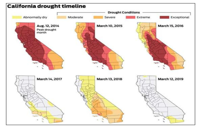
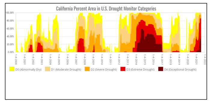
| [51] | United States Drought Monitor (USDM) 2014 to 2019 California Drought Trends, 2019. Available from: https://droughtmonitor.unl.edu/Maps/MapArchive.aspx |
| [52] |
Diffenbaugh NS, Swain DL, Touma D (2015) Anthropogenic warming has increased drought risk in California. PNAS 112: 3931–3936. https://doi.org/10.1073/pnas.1422385112 doi: 10.1073/pnas.1422385112
|
| [53] | Mirchi A, Madani K, Roos M, et al. (2013) Climate change impacts on California's Water Resources. Drought Arid Semi-arid Reg 301–319. https://doi.org/10.1007/978-94-007-6636-5_17 |
| [54] |
Thomas BF, Famiglietti JS, Landerer FW, et al. (2017) GRACE Groundwater Drought Index: Evaluation of California Central Valley groundwater drought. Remote Sens Environ 198: 384–392. https://doi.org/10.1016/j.rse.2017.06.026 doi: 10.1016/j.rse.2017.06.026
|
| [55] |
Faunt CC, Sneed M, Traum J, et al. (2016) Water Availability and Land Subsidence in the Central Valley, California, USA. Hydrogeol J 24: 675–684. https://doi.org/10.1007/s10040-015-1339-x doi: 10.1007/s10040-015-1339-x
|
| [56] |
Langridge R, Daniels B (2017) Accounting for Climate Change and Drought in Implementing Sustainable Groundwater Management. Water Resour Manage 31: 3287–3298. https://doi.org/10.1007/s11269-017-1607-8 doi: 10.1007/s11269-017-1607-8
|
| [57] | Xiao M, Koppa A, Mekonnen Z, et al. (2017) How much groundwater did California's Central Valley lose during the 2012–2016 drought? Geophys Res Letters 44: 4872–4879. https://doi.org/10.1002/2017GL073333 |
| [58] | Upper Santa Ana River Watershed: Integrated Regional Water Management Plan, 2015. Available from: https://www.sbvwcd.org/docman-projects/upper-santa-ana-integrated-regional-water-management-plan/3802-usarw-irwmp-2015-ch1-9-final/file |
| [59] |
Brown AE, Zhang L, McMahon TA, et al. (2005) A review of paired catchment studies for determining changes in water yield resulting from alterations in vegetation. J Hydrol 310: 28–61. https://doi.org/10.1016/j.jhydrol.2004.12.010 doi: 10.1016/j.jhydrol.2004.12.010
|
| [60] |
Anderson DM, Gilbert PM, Burkholder JM (2002) Harmful algal blooms and eutrophication: Nutrient sources, composition, and consequences. Estuaries 25: 704–726. https://doi.org/10.1007/BF02804901 doi: 10.1007/BF02804901
|
| [61] | California Water Quality Monitoring Council (CAWQ). Harmful Algal Bloom Incident Reports Map, 2020. Available from: https://mywaterquality.ca.gov/habs/where/freshwater_events.html |
| [62] | California Water News Daily (WND). Blue-Green Algae Blooming Throughout California, 2019. Available from: http://californiawaternewsdaily.com/drought/blue-green-algae-blooming-throughout-california/ |
| [63] |
Kiparsky M, Milman A, Owen D, et al. (2017) The Importance of Institutional Design for Distributed Local-level Governance of Groundwater: The Case of California's Sustainable Groundwater Management Act. Water 9: 755–772. https://doi.org/10.3390/w9100755 doi: 10.3390/w9100755
|
| [64] |
Thomas BF (2018) Sustainability indices to evaluate groundwater adaptive management: a case study in California (USA) for the Sustainable Groundwater Management Act. Hydrogeol J 27: 239–248. https://doi.org/10.1007/s10040-018-1863-6 doi: 10.1007/s10040-018-1863-6
|
| [65] | Association of California Water Agencies (ACAWA), 2021. Available from: https://www.acwa.com/our-work/protecting-water-at-its-source/ |
| [66] | California Public Policy Institute (CAPPI) Protecting Headwaters, 2021. Available from: https://www.ppic.org/content/pubs/report/R_1016JM4R.pdf |
| [67] | California Water Education Foundation (CWEF) Headwaters, 2021. Available from: https://www.watereducation.org/aquapedia-background/headwaters |
| [68] | State Water Board (SWB) A Primer on stream and river protection for the regulator and program manager, 2003. Available from: https://www.waterboards.ca.gov/rwqcb2/water_issues/programs/stream_wetland/streamprotectioncircular.pdf |
| [69] | Public Policy Institute of California (PPIC) California's Water, 2016. Available from: https://www.ppic.org/content/pubs/report/R_1016WPCBKR.pdf |
| [70] |
Alexander RB, Boyer EW, Smith RA, et al. (2007) The Role of Headwater Streams in Downstream Water Quality. J Amer Water Resor Assoc 43: 41–59. https://doi.org/10.1111/j.1752-1688.2007.00005.x doi: 10.1111/j.1752-1688.2007.00005.x
|
| [71] | United States Geological Survey (USGS) Geologic Map of the San Bernardino North 7.5' quadrangle, San Bernardino County, California, 2001. Available from: https://pubs.er.usgs.gov/publication/ofr01131 |
| [72] | National Oceanic and Atmospheric Administration (NOAA) Climate types, 2021. Available from: https://www.weather.gov/jetstream/climates |
| [73] | United States Climate Data (USCD), 2019. Available from: https://www.usclimatedata.com/climate/san-bernardino/california/united-states/usca0978 |
| [74] | United States Environmental Protection Agency (EPA) Viewing WATERS Data using Google Earth, 2017. Available from: https://www.epa.gov/waterdata/viewing-waters-data-using-google-earth |
| [75] | State Water Board (SWB) Santa Ana River Water Right Applications For Supplemental Water Supply Draft Environmental Impact Report, 2004. Available from: https://www.waterboards.ca.gov/waterrights/water_issues/programs/hearings/santa_ana_river/docs/deir_appendixa.pdf |
| [76] | California Water Education Foundation (CWEF) Headwaters, 2021. Available from: https://www.watereducation.org/aquapedia/santa-ana-river |
| [77] | Santa Ana Watershed Project Authority One Water One Watershed 2.0 Plan, 2021. Available from: https://sawpa.org/owow/owow-irwm-plans/owow-2-0-plan/ |
| [78] | Multi-Resolution Land Characteristics Consortium (MRLC). Multi-Resolution Land Characteristics Consortium National Land Cover Dataset, 2019. Available from: https://www.mrlc.gov |
| [79] | Weather Underground Upper Waterman Canyon. Available from: https://www.wunderground.com/?ID=KCASANBE93 |
| [80] | San Bernardino Valley Municipal Water District (SBVMWD) 2019. Available from: https://www.sbvmwd.com |
| [81] | Crestline Sanitation District (CSD). 2019. Available from: http://www.crestlinesanitation.com |
| [82] | Abu-Baker S, Frazier C, Frazier N, et al. (2016) Engaging Freshman Undergraduate Students in Faculty Environmental Science Research: Testing the Local Surface Waters for Nitrate, Phosphate, and Ammonium Ions Using Two Affordable Methods as an Example. Green Sustain Chem 6. https://doi.org/10.4236/gsc.2016.63014 |
| [83] |
Khatoon N, Khan AH, Rehman M, et al. (2013) Correlation Study For the Assessment of Water Quality and Its Parameters of Ganga River, Kanpur, Uttar Pradesh, India. J Applied Chem 5: 80–90. https://doi.org/10.9790/5736-0538090 doi: 10.9790/5736-0538090
|
| [84] |
Vega M, Pardo R, Barrado E, et al. (1998) Assessment of Seasonal and Polluting Effects on the Quality of River Water by Exploratory Data Analysis. Water Res 32: 3581–3592. https://doi.org/10.1016/S0043-1354(98)00138-9 doi: 10.1016/S0043-1354(98)00138-9
|
| [85] |
Varol M, Gö kot B, Bekleyen A, et al. (2012) Spatial and Temporal Variations in Surface Water Quality of the Dam Reservoirs in the Tigris River Basin, Turkey. Catena 92: 11–21. https://doi.org/10.1016/j.catena.2011.11.013 doi: 10.1016/j.catena.2011.11.013
|
| [86] | United States Environmental Protection Agency (EPA), Guidelines Establishing Test Procedures for the Analysis of Pollutants; Analytical Methods for Biological Pollutants in Ambient Water; Final Rule, 2003. Available from: https://123.idexx.com/resource-library/water/water-reg-article5AP-v2.pdf |
| [87] | Clean Water Team, Division of Water Quality, California State Water Resources Control Board (SWRCB). 2004 Turbidity Fact Sheet, 2004. Available from: https://www.waterboards.ca.gov/water_issues/programs/swamp/docs/cwt/guidance/3150en.pdf |
| [88] | United States Environmental Protection Agency (EPA) E. Coli and Enterococci, 2018. Available from: https://www.epa.gov/sites/production/files/2015-09/documents/eColi.pdf |
| [89] | United States Environmental Protection Agency (EPA), National Cost Analysis for Drinking Water Regulations, 2018. Available from: https://www.epa.gov/dwregdev/national-cost-analysis-drinking-water-regulations |
| [90] | California State Water Board, Stream Temperature Indices, Thresholds, and Standards Used to Protect Coho Salmon Habitat: A Rivew, 2002. Available from: https://www.waterboards.ca.gov/water_issues/programs/tmdl/records/region_1/2006/ref33.pdf |
| [91] | Water Quality Control Plan (WQCP) Lahontan Region North and South Basins, State of California Regional Water Quality Control Board Lahontan Region, 2015. Available from: https://www.epa.gov/sites/production/files/2015-09/documents/ca6-north-south.pdf |
| [92] |
Mallin MA, Turner MIH, McIver MR, et al. (2016) Significant Reduction of Fecal Bacteria and Suspended Solids Loading by Coastal Best Management Practices. J Coastal Res 32: 923–931. https://doi.org/10.2112/JCOASTRES-D-15-00195.1 doi: 10.2112/JCOASTRES-D-15-00195.1
|
| [93] | United States Geological Survey (USGS), Methods for Computing Water Quality Using Regression Analysis, 2019. Available from: http://nrtwq.usgs.gov/md/methods/ |
| [94] | Yuncong L, Migliaccio K (2011) Water Quality Concepts, Sampling, & Analysis. Boca Raton, FL. Taylor Group. |
| [95] |
Ding S, Zhang Y, Liu B, et al. (2013) Effects of riparian land use on water quality and fish communities in the headwater stream of the Taizi River in China. Front Environ Sci Eng 7: 699–708. https://doi.org/10.1007/s11783-013-0528-x doi: 10.1007/s11783-013-0528-x
|
| [96] |
Mallin MA, Kathleen EW, Esham EC, et al. (2000) Effect of Human Development on Bacteriological Water Quality in Coastal Watersheds. Ecol Appl 10: 1047–1056. https://doi.org/10.1890/1051-0761(2000)010[1047:EOHDOB]2.0.CO;2 doi: 10.1890/1051-0761(2000)010[1047:EOHDOB]2.0.CO;2
|
| [97] | United States Geological Survey (USGS) California Drought, 2019. Available from: https://ca.water.usgs.gov/california-drought/index.html |
| [98] |
Winter TC (2017) The Role of Ground Water Streamflow in Headwater Areas and in Maintaining Base Flow. J Am Water Resour Assoc 43: 15–25. https://doi.org/10.1111/j.1752-1688.2007.00003.x doi: 10.1111/j.1752-1688.2007.00003.x
|
| [99] |
Avanzi F, Rungee J, Maurer T, et al. (2020) Climate elasticity of evapotranspiration shifts the water balance of Mediterranean climate during multi-year drought. Hydrol Earth Syst Sci 24: 4317–4337. https://doi.org/10.5194/hess-24-4317-2020 doi: 10.5194/hess-24-4317-2020
|
| [100] |
Walsh CJ, Roy AH, Feminella JW, et al. (2005) The Urban Stream Syndrome: Current Knowledge and the Search for a Cure. J North Amer Benthological Soc 24: 706–723. https://doi.org/10.1899/04-028.1 doi: 10.1899/04-028.1
|
| [101] |
Wear DN, Turner MG, Naiman RJ (1998) Land Cover Along an Urban-Rural Gradient: Implications for Water Quality. Ecol Appl 8: 619–630. https://doi.org/10.1890/1051-0761(1998)008[0619:LCAAUR]2.0.CO;2 doi: 10.1890/1051-0761(1998)008[0619:LCAAUR]2.0.CO;2
|
| [102] |
Pratt B, Chang H (2012). Effects of land cover, topography, and built structure on seasonal water quality at multiple spatial scales. J Hazard Mater 209–210: 48–58. https://doi.org/10.1016/j.jhazmat.2011.12.068 doi: 10.1016/j.jhazmat.2011.12.068
|
| [103] |
Gasith A, Resh VH (1999) Streams in Mediterranean Climate Regions: Abiotic Influences and Biotic Responses to Predictable Seasonal Events. Annu Rev Ecol Syst 30: 51–81. https://doi.org/10.1146/annurev.ecolsys.30.1.51 doi: 10.1146/annurev.ecolsys.30.1.51
|
| [104] |
Weber G, Honecker U, Jochen K (2020) Nitrate dynamics in springs and headwater streams with agricultural catchments in southwestern Germany. Sci Total Environ 722: 137858. https://doi.org/10.1016/j.scitotenv.2020.137858 doi: 10.1016/j.scitotenv.2020.137858
|
| [105] | United States Environmental Protection Agency (EPA) The effects of climate change on water resources and programs, 2021. Available from: https://cfpub.epa.gov/watertrain/moduleFrame.cfm?parent_object_id=2456&object_id=2459#:~:text=The%20Effect%20on%20Water%20Resources,temperatures%20to%20increase%20as%20well.&text=Lower%20levels%20of%20dissolved%20oxygen,increases%2C%20dissolved%20oxygen%20levels%20decrease |
| [106] | United States Environmental Protection Agency (EPA) Introduction to watershed ecology, 2021. Available from: https://cfpub.epa.gov/watertrain/moduleFrame.cfm?parent_object_id=593 |
| [107] |
Carpenter SR, Caraco NF, Correll DL, et al. (1998) Nonpoint Pollution of Surface Waters with Phosphorus and Nitrogen. Ecol Appl 8: 559–568. https://doi.org/10.1890/1051-0761(1998)008[0559:NPOSWW]2.0.CO;2 doi: 10.1890/1051-0761(1998)008[0559:NPOSWW]2.0.CO;2
|
| [108] |
De Roos AJ, Zahm SH, Cantor KP, et al. (2003) Integrative assessment of multiple pesticides as risk factors for non-Hodgkin's lymphoma among men. Occup Environ Med 60: e11. https://doi.org/10.1136/oem.60.9.e11 doi: 10.1136/oem.60.9.e11
|
| [109] |
Mosley LM (2015) Drought impacts on the water quality of freshwater systems; review and integration. Earth-Sci Rev 140: 203–214. https://doi.org/10.1016/j.earscirev.2014.11.010 doi: 10.1016/j.earscirev.2014.11.010
|
| [110] |
Barrett ME (2005) Performance Comparison of Structural Stormwater Best Management Practices. Water Environ Res 77: 78–86. https://doi.org/10.2175/106143005X41654 doi: 10.2175/106143005X41654
|
| [111] |
Commings KJ, Booth DB, Horner RR (2000) Storm Water Pollutant Removal by Two Wet Ponds in Bellevue, Washington. J Environ 126: 321–330. https://doi.org/10.1061/(ASCE)0733-9372(2000)126:4(321) doi: 10.1061/(ASCE)0733-9372(2000)126:4(321)
|
| [112] |
Roy, AH, Rhea LK, Mayer AL, et al. (2014) St. Amand, A. How Much Is Enough? Minimal Resources of Water Quality and Stream Biota to Partial Retrofit Stormwater Management in a Suburban Neighborhood. PLoS ONE 9: 1–14. https://doi.org/10.1371/journal.pone.0085011 doi: 10.1371/journal.pone.0085011
|
| [113] |
Ice G, Sugden B (2003) Summer dissolved oxygen concentrations in forested streams of Northern Louisiana. South J Appl For 27: 92–99. https://doi.org/10.1093/sjaf/27.2.92 doi: 10.1093/sjaf/27.2.92
|
| [114] |
Van Vliet MTH, Zwolsman JJG (2008) Impact of Summer Droughts on the Water Quality of the Meuse River. J Hydrol 353: 1–17. https://doi.org/10.1016/j.jhydrol.2008.01.001 doi: 10.1016/j.jhydrol.2008.01.001
|
| [115] |
Liu BW, Wang MH, Chen TL, et al. (2020) Establishment and implementation of green infrastructure practice for healthy watershed management: Challenges and perspectives. Water Energy Nexus 3: 186–197. https://doi.org/10.1016/j.wen.2020.05.003 doi: 10.1016/j.wen.2020.05.003
|
| [116] | United States Forest Service (USFS), Sediment loads and erosion in forest headwater streams of the Sierra Nevada, California, 2012. Available from: https://www.fs.usda.gov/treesearch/pubs/41235 |
| [117] | Fischer ME, Irlenbusch B, Sadrieh A (2004) An intergenerational pool resource experiment J Environ Econ Mange 48: 811–836. https://doi.org/10.1016/j.jeem.2003.12.002 |
| [118] | Ostrom E (2005) Understanding Institutional Diversity, Princeton NJ: Princeton University Press. |
| [119] | Slough T, Rubenson D, Levy R, et al. (2021) Adoption of community monitoring improves common pool resource management across contexts. PNAS 118. https://doi.org/10.1073/pnas.2015367118 |
Figures(9) / Tables(6)

Jennifer B Alford, Jose A Mora. Factors influencing chronic semi-arid headwater stream impairments: a southern California case study[J]. AIMS Geosciences, 2022, 8(1): 98-126. doi: 10.3934/geosci.2022007


 DownLoad: