Research on reinforcement learning based on PPO algorithm for human-machine intervention in autonomous driving

Gaosong Shi; Qinghai Zhao; Jirong Wang; Xin Dong; Gaosong Shi; Qinghai Zhao; Jirong Wang; Xin Dong

doi:10.3934/era.2024111

Electronic Research Archive

2024, Volume 32, Issue 4: 2424-2446. doi: 10.3934/era.2024111

Previous Article Next Article

Research article Special Issues

Research on reinforcement learning based on PPO algorithm for human-machine intervention in autonomous driving

1.
College of Mechanical and Electrical Engineering, Qingdao University, Qingdao 266071, China
2.
National Engineering Research Center for Intelligent Electrical Vehicle Power System, Qingdao 266071, China

Received: 05 November 2023 Revised: 12 March 2024 Accepted: 19 March 2024 Published: 26 March 2024

Given the current limitations in intelligence and processing capabilities, machine learning systems are yet unable to fully tackle diverse scenarios, thereby restricting their potential to completely substitute for human roles in practical applications. Recognizing the robustness and adaptability demonstrated by human drivers in complex environments, autonomous driving training has incorporated driving intervention mechanisms. By integrating these interventions into Proximal Policy Optimization (PPO) algorithms, it becomes possible for drivers to intervene and rectify vehicles' irrational behaviors when necessary, during the training process, thereby significantly accelerating the enhancement of model performance. A human-centric experiential replay mechanism has been developed to increase the efficiency of utilizing driving intervention data. To evaluate the impact of driving intervention on the performance of intelligent agents, experiments were conducted across four distinct intervention frequencies within scenarios involving lane changes and navigation through congested roads. The results demonstrate that the bespoke intervention mechanism markedly improves the model's performance in the initial stages of training, enabling it to overcome local optima through timely driving interventions. Although an increase in intervention frequency typically results in improved model performance, an excessively high intervention rate can detrimentally affect the model's efficiency. To assess the practical applicability of the algorithm, a comprehensive testing scenario that includes lane changes, traffic signals, and congested road sections was devised. The performance of the trained model was evaluated under various traffic conditions. The outcomes reveal that the model can adapt to different traffic flows, successfully and safely navigate the testing segment, and maintain speeds close to the target. These findings highlight the model's robustness and its potential for real-world application, emphasizing the critical role of human intervention in enhancing the safety and reliability of autonomous driving systems.
- autonomous driving,
- driving intervention,
- experience replay,
- lane-changing,
- lane-following
Citation: Gaosong Shi, Qinghai Zhao, Jirong Wang, Xin Dong. Research on reinforcement learning based on PPO algorithm for human-machine intervention in autonomous driving[J]. Electronic Research Archive, 2024, 32(4): 2424-2446. doi: 10.3934/era.2024111

Related Papers:

Abstract

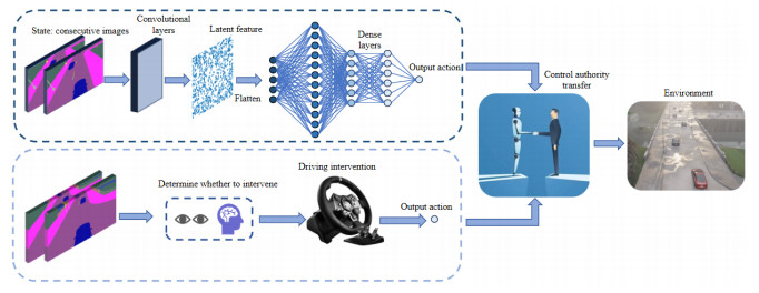
Given the current limitations in intelligence and processing capabilities, machine learning systems are yet unable to fully tackle diverse scenarios, thereby restricting their potential to completely substitute for human roles in practical applications. Recognizing the robustness and adaptability demonstrated by human drivers in complex environments, autonomous driving training has incorporated driving intervention mechanisms. By integrating these interventions into Proximal Policy Optimization (PPO) algorithms, it becomes possible for drivers to intervene and rectify vehicles' irrational behaviors when necessary, during the training process, thereby significantly accelerating the enhancement of model performance. A human-centric experiential replay mechanism has been developed to increase the efficiency of utilizing driving intervention data. To evaluate the impact of driving intervention on the performance of intelligent agents, experiments were conducted across four distinct intervention frequencies within scenarios involving lane changes and navigation through congested roads. The results demonstrate that the bespoke intervention mechanism markedly improves the model's performance in the initial stages of training, enabling it to overcome local optima through timely driving interventions. Although an increase in intervention frequency typically results in improved model performance, an excessively high intervention rate can detrimentally affect the model's efficiency. To assess the practical applicability of the algorithm, a comprehensive testing scenario that includes lane changes, traffic signals, and congested road sections was devised. The performance of the trained model was evaluated under various traffic conditions. The outcomes reveal that the model can adapt to different traffic flows, successfully and safely navigate the testing segment, and maintain speeds close to the target. These findings highlight the model's robustness and its potential for real-world application, emphasizing the critical role of human intervention in enhancing the safety and reliability of autonomous driving systems.

References

[1]	I. Yaqoob, L. U. Khan, S. M. A. Kazmi, M. Imran, N. Guizani, C. S. Hong, Autonomous driving cars in smart cities: Recent advances, requirements, and challenges, IEEE Network, 34 (2020), 174–181. https://doi.org/10.1109/MNET.2019.1900120
[2]	B. R. Kiran, I. Sobh, V. Talpaert, P. Mannion, A. A. Sallab, S. Yogamani, et al., Deep reinforcement learning for autonomous driving: a survey, IEEE Trans. Intell. Transp. Syst., 23 (2022), 4909–4926. https://doi.org/10.1109/TITS.2021.3054625 doi: 10.1109/TITS.2021.3054625
[3]	L. Anzalone, P. Barra, S. Barra, A. Castiglione, M. Nappi, An end-to-end curriculum learning approach for autonomous driving scenarios, IEEE Trans. Intell. Transp. Syst., 23 (2022), 19817–19826. https://doi.org/10.1109/TITS.2022.3160673 doi: 10.1109/TITS.2022.3160673
[4]	J. Hua, L. Zeng, G. Li, Z. Ju, Learning for a Robot: Deep reinforcement learning, imitation learning, transfer learning, Sensors, 21 (2021), 1278. https://doi.org/10.3390/s21041278
[5]	K. Makantasis, M. Kontorinaki, I. Nikolos, Deep reinforcement‐learning‐based driving policy for autonomous road vehicles, IET Intell. Transp. Syst., 14 (2019), 13–24. https://doi.org/10.1049/iet-its.2019.0249 doi: 10.1049/iet-its.2019.0249
[6]	L. L. Mero, D. Yi, M. Dianati, A. Mouzakitis, A survey on imitation learning tech-niques for end-to-end autonomous vehicles, IEEE Trans. Intell. Transp. Syst., 23 (2022), 14128–14147. https://doi.org/10.1109/TITS.2022.3144867 doi: 10.1109/TITS.2022.3144867
[7]	A. Hussein, M. M. Gaber, E. Elyan, C. Jayne, Imitation learning: A survey of learning methods, ACM Comput. Surv., 50 (2017), 1–35. https://doi.org/10.1145/3054912 doi: 10.1145/3054912
[8]	Y. Peng, G. Tan, H. Si, RTA-IR: A runtime assurance framework for behavior planning based on imitation learning and responsibility-sensitive safety model, Expert Syst. Appl., 232 (2023). https://doi.org/10.1016/j.eswa.2023.120824
[9]	H. M. Eraqi, M. N. Moustafa, J. Honer, Dynamic conditional imitation learning for autonomous driving, IEEE Trans. Intell. Transp. Syst., 23 (2022), 22988–23001. https://doi.org/10.1109/TITS.2022.3214079 doi: 10.1109/TITS.2022.3214079
[10]	S. Teng, L. Chen, Y. Ai, Y. Zhou, Z. Xuanyuan, X. Hu, Hierarchical interpretable imitation learning for end-to-end autonomous driving, IEEE Trans. Intell. Transp. Syst., 8 (2023), 673–683. https://doi.org/10.1109/TIV.2022.3225340 doi: 10.1109/TIV.2022.3225340
[11]	J. Ahn, M. Kim, J. Park, Autonomous driving using imitation learning with a look ahead point for semi-structured environments, Sci. Rep., 12 (2022), 21285. https://doi.org/10.1038/s41598-022-23546-6 doi: 10.1038/s41598-022-23546-6
[12]	B. Zheng, S. Verma, J. Zhou, I. W. Tsang, F. Chen, Imitation learning: Progress, taxonomies and challenges, IEEE Trans. Neural Networks Learn. Syst., (2022), 1–16. https://doi.org/10.1109/TNNLS.2022.3213246
[13]	Z. Wu, K. Qiu, H. Gao, Driving policies of V2X autonomous vehicles based on reinforcement learning methods, IET Intell. Transp. Syst., 14 (2020), 331–337. https://doi.org/10.1049/iet-its.2019.0457 doi: 10.1049/iet-its.2019.0457
[14]	C. You, J. Lu, D. Filev, P. Tsiotras, Advanced planning for autonomous vehicles using reinforcement learning and deep inverse reinforcement learning, Rob. Auton. Syst., 114 (2019), 1–18. https://doi.org/10.1016/j.robot.2019.01.003 doi: 10.1016/j.robot.2019.01.003
[15]	D. Zhang, X. Han, C. Deng, Review on the research and practice of deep learning and reinforcement learning in smart grids, CSEE J. Power Energy Syst., 4 (2018), 362–370. https://doi.org/10.17775/CSEEJPES.2018.00520 doi: 10.17775/CSEEJPES.2018.00520
[16]	Y. H. Khalil, H. T. Mouftah, Exploiting multi-modal fusion for urban autonomous driving using latent deep reinforcement learning, IEEE Trans. Veh. Technol., 72 (2023), 2921–2935. https://doi.org/10.1109/TVT.2022.3217299 doi: 10.1109/TVT.2022.3217299
[17]	H. Zhang, Y. Lin, S. Han, K. Lv, Lexicographic actor-critic deep reinforcement learning for urban autonomous driving, IEEE Trans. Veh. Technol., 72 (2023), 4308–4319. https://doi.org/10.1109/TVT.2022.3226579 doi: 10.1109/TVT.2022.3226579
[18]	Z. Du, Q. Miao, C. Zong, Trajectory planning for automated parking systems using deep reinforcement learning, Int. J. Automot. Technol., 21 (2020), 881–887. https://doi.org/10.1007/s12239-020-0085-9 doi: 10.1007/s12239-020-0085-9
[19]	E. O. Neftci, B. B. Averbeck, Reinforcement learning in artificial and biological systems, Nat. Mach. Intell., 1 (2019), 133–143. https://doi.org/10.1038/s42256-019-0025-4 doi: 10.1038/s42256-019-0025-4
[20]	M. L. Littman, Reinforcement learning improves behavior from evaluative feedback, Nature, 521 (2015), 445–451. https://doi.org/10.1038/nature14540 doi: 10.1038/nature14540
[21]	E. O. Neftci, B. B. Averbeck, Reinforcement learning in artificial and biological systems, Nat. Mach. Intell., 1 (2019), 133–143. https://doi.org/10.1038/s42256-019-0025-4 doi: 10.1038/s42256-019-0025-4
[22]	C. Zhu, Y. Cai, J. Zhu, C. Hu, J. Bi, GR(1)-guided deep reinforcement learning for multi-task motion planning under a stochastic environment, Electronics, 11 (2022), 3716. https://doi.org/10.3390/electronics11223716 doi: 10.3390/electronics11223716
[23]	J. Schulman, F. Wolski, P. Dhariwal, A. Radford, O. Klimov, Proximal policy optimization algorithms, preprint, arXiv: 1707.06347. https://doi.org/10.48550/arXiv.1707.06347
[24]	W. Guan, Z. Cui, X. Zhang, Intelligent smart marine autonomous surface ship decision system based on improved PPO algorithm, Sensors, 22 (2022), 5732. https://doi.org/10.3390/s22155732 doi: 10.3390/s22155732
[25]	J. Han, K. Jo, W. Lim, Y. Lee, K. Ko, E. Sim, et al., Reinforcement learning guided by double replay memory, J. Sens., 2021 (2021), 1–8. https://doi.org/10.1155/2021/6652042 doi: 10.1155/2021/6652042
[26]	H. Liu, A. Trott, R. Socher, C. Xiong, Competitive experience replay, preprint, arXiv: 1902.00528. https://doi.org/10.48550/arXiv.1902.00528
[27]	X. Wang, H. Xiang, Y. Cheng, Q. Yu, Prioritised experience replay based on sample optimization, J. Eng., 2020 (2020), 298–302. https://doi.org/10.1049/joe.2019.1204 doi: 10.1049/joe.2019.1204
[28]	A. Karalakou, D. Troullinos, G. Chalkiadakis, M. Papageorgiou, Deep reinforcement learning reward function design for autonomous driving in lane-free traffic, Systems, 11 (2023), 134. https://doi.org/10.3390/systems11030134 doi: 10.3390/systems11030134
[29]	B. Geng, J. Ma, S. Zhang, Ensemble deep learning-based lane-changing behavior prediction of manually driven vehicles in mixed traffic environments, Electron. Res. Arch., 31 (2023), 6216–6235. https://doi.org/10.3934/era.2023315 doi: 10.3934/era.2023315
[30]	M. Andrychowicz, F. Wolski, A. Ray, J. Schneider, R. Fong, Hindsight experience replay, preprint, arXiv: 1707.01495.
[31]	J. Wu, Z. Huang, Z. Hu, C. Lu, Toward human-in-the-loop AI: Enhancing deep reinforcement learning via real-time human intervention for autonomous driving, Engineering, 21(2023), 75–91. https://doi.org/10.1016/j.eng.2022.05.017 doi: 10.1016/j.eng.2022.05.017
[32]	F. Pan, H. Bao, Preceding vehicle following algorithm with human driving characteristics, Proc. Inst. Mech. Eng., Part D: J. Automob. Eng., 235 (2021), 1825–1834. https://doi.org/10.1177/0954407020981546 doi: 10.1177/0954407020981546
[33]	Y. Zhou, R. Fu, C. Wang, Learning the car-following behavior of drivers using maximum entropy deep inverse reinforcement learning, J. Adv. Transp. , 2020 (2020), 1–13. https://doi.org/10.1155/2020/4752651 doi: 10.1155/2020/4752651
[34]	S. Lee, D. Ngoduy, M. Keyvan-Ekbatani, Integrated deep learning and stochastic car-following model for traffic dynamics on multi-lane freeways, Transp. Res. Part C Emerging Technol., 106 (2019), 360–377. https://doi.org/10.1016/j.trc.2019.07.023 doi: 10.1016/j.trc.2019.07.023

Reader Comments

Your name:*

Email:*
© 2024 the Author(s), licensee AIMS Press. This is an open access article distributed under the terms of the Creative Commons Attribution License (http://creativecommons.org/licenses/by/4.0)