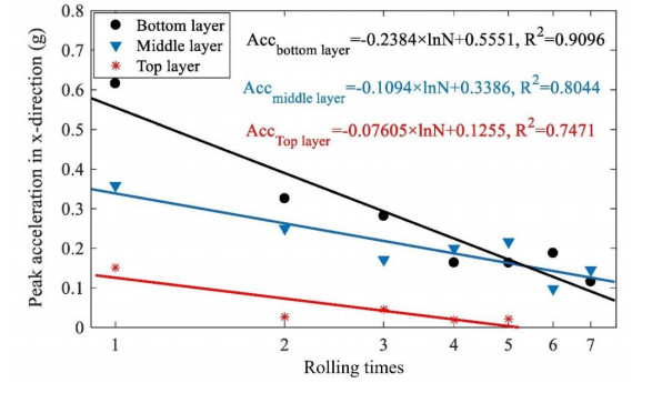
Asphalt mixture is composed of asphalt binder with aggregates of different sizes and compacted under static or dynamic forces. In practical engineering, compaction is a critical step in asphalt pavement construction to determine the quality and service life of pavement. Since the dynamic response characteristics of asphalt pavement can reflect the compaction state of asphalt mixture in the process of compaction, the establishment of the relationship between dynamic response characteristics and compaction degree is definitely significant. In this paper, a series of vibration sensors were adopted to capture the dynamic response signal of the vibration drum and asphalt mixture in the process of vibrating compaction for different surface courses of pavement. Then, the change regulations of vibration acceleration of vibrating drum and asphalt mixture were analyzed, and the quantitative linear relationship was established between accelerations of vibrating drum and asphalt pavement compactness. Further, the concept of evaluation unit (i.e., within 2 meters along the driving direction of the roller) and prediction method of compaction degree were proposed as well. The results showed that under the same vibration compaction condition, the compaction degree values of the top, middle and bottom layers have obvious differences, which should be taken seriously into consideration in the compaction process. Meanwhile, there is little difference which respectively are 2.8, 1.3 and 0.82% for the top, middle and bottom layers between the compaction degrees obtained by the proposed method and measured test. Therefore, the average value of the acceleration peak value of vibration drum within the evaluation unit can be adopted as the characterization index of the compaction degree of asphalt pavement. The investigation of this study can provide the technical reference for compaction control of asphalt pavement to a large extent.
Citation: Hongyu Shan, Han-Cheng Dan, Shiping Wang, Zhi Zhang, Renkun Zhang. Investigation on dynamic response and compaction degree characterization of multi-layer asphalt pavement under vibration rolling[J]. Electronic Research Archive, 2023, 31(4): 2230-2251. doi: 10.3934/era.2023114
Asphalt mixture is composed of asphalt binder with aggregates of different sizes and compacted under static or dynamic forces. In practical engineering, compaction is a critical step in asphalt pavement construction to determine the quality and service life of pavement. Since the dynamic response characteristics of asphalt pavement can reflect the compaction state of asphalt mixture in the process of compaction, the establishment of the relationship between dynamic response characteristics and compaction degree is definitely significant. In this paper, a series of vibration sensors were adopted to capture the dynamic response signal of the vibration drum and asphalt mixture in the process of vibrating compaction for different surface courses of pavement. Then, the change regulations of vibration acceleration of vibrating drum and asphalt mixture were analyzed, and the quantitative linear relationship was established between accelerations of vibrating drum and asphalt pavement compactness. Further, the concept of evaluation unit (i.e., within 2 meters along the driving direction of the roller) and prediction method of compaction degree were proposed as well. The results showed that under the same vibration compaction condition, the compaction degree values of the top, middle and bottom layers have obvious differences, which should be taken seriously into consideration in the compaction process. Meanwhile, there is little difference which respectively are 2.8, 1.3 and 0.82% for the top, middle and bottom layers between the compaction degrees obtained by the proposed method and measured test. Therefore, the average value of the acceleration peak value of vibration drum within the evaluation unit can be adopted as the characterization index of the compaction degree of asphalt pavement. The investigation of this study can provide the technical reference for compaction control of asphalt pavement to a large extent.

| [1] |
S. C. Zhu, X. D. Li, H. Y. Wang, D. X. Yu, Development of an automated remote asphalt paving quality control system, Transp. Res. Record, 2672 (2018), 28–39. https://doi.org/10.1177/0361198118758690 doi: 10.1177/0361198118758690

|
| [2] |
F. Beainy, S. Commuri, M. Zaman, Dynamical response of vibratory rollers during the compaction of asphalt pavements, J. Eng. Mech., 140 (2014), 04014039. https://doi.org/10.1061/(ASCE)EM.1943-7889.0000730 doi: 10.1061/(ASCE)EM.1943-7889.0000730
|
| [3] |
R. Micaelo, C. Azevedo, J. Ribeiro, Hot-mix asphalt compaction evaluation with field test, Balt. J. Road Bridge Eng., 9 (2014), 306–316. https://doi.org/10.3846/BJRBE.2014.37 doi: 10.3846/BJRBE.2014.37
|
| [4] |
T. Jia, T. He, Z. D. Qian, J. Lv, K. X. Cao, An improved low-cost continuous compaction detection method for the construction of asphalt pavement, Adv. Civil Eng., 2019 (2019), 4528230. https://doi.org/10.1155/2019/4528230 doi: 10.1155/2019/4528230
|
| [5] | Ministry of Transport of the People's Republic of China, Standard Test Methods for Bitumen and Bituminous Mixtures for Highway Engineering, JTG E20, China Communications Press, Beijing, China, 2019. |
| [6] |
H. C. Dan, Z. Zhang, J. Q. Chen, H. Wang, Numerical simulation of an indirect tensile test for asphalt mixtures using discrete element method software, J. Mater. Civ. Eng., 30 (2018), 04018067. https://doi.org/10.1061/(ASCE)MT.1943-5533.0002252 doi: 10.1061/(ASCE)MT.1943-5533.0002252
|
| [7] |
H. C. Dan, J. W. Tan, J. Q. Chen, Temperature distribution of asphalt bridge deck pavement with groundwater circulation temperature control system under high- and low temperature conditions, Road Mater. Pavement Des., 20 (2019), 528–553. https://doi.org/10.1080/14680629.2017.1397048 doi: 10.1080/14680629.2017.1397048
|
| [8] |
H. C. Dan, J. W. Tan, Y. F. Du, J. M. Cai, Simulation and optimization of road deicing salt usage based on Water-Ice-Salt Model, Cold Reg. Sci. Technol., 169 (2020), 102917. https://doi.org/10.1016/j.coldregions.2019.102917 doi: 10.1016/j.coldregions.2019.102917
|
| [9] |
Y. Q. Tan, H. P. Wang, S. J. Mao, H. N. Xu, Quality control of asphalt pavement compaction using fibre Bragg grating sensing technology, Constr. Build. Mater., 54 (2014), 53–59. https://doi.org/10.1016/j.conbuildmat.2013.12.032 doi: 10.1016/j.conbuildmat.2013.12.032
|
| [10] |
Q. Xu, G. K. Chang, Experimental and numerical study of asphalt material geospatial heterogeneity with intelligent compaction technology on roads, Constr. Build. Mater., 72 (2014), 189–198. https://doi.org/10.1016/j.conbuildmat.2014.09.00 doi: 10.1016/j.conbuildmat.2014.09.00
|
| [11] |
J. S. Chen, B. S. Huang, X. Shu, C. C. Hu, DEM simulation of laboratory compaction of asphalt mixtures using an open source code, J. Mater. Civ. Eng., 27 (2015), 04014130. https://doi.org/10.1061/(ASCE)MT.1943-5533.0001069 doi: 10.1061/(ASCE)MT.1943-5533.0001069
|
| [12] |
G. K. Chang, K. Mohanraj, W. A. Stone, D. J. Oesch, V. Gallivan, Leveraging intelligent compaction and thermal profiling technologies to improve asphalt pavement construction quality: A case study, Transp. Res. Record, 2672 (2018), 48–56. https://doi.org/10.1177/0361198118758285 doi: 10.1177/0361198118758285
|
| [13] |
P. Shangguan, I. Al-Qadi, A. Coenen, Algorithm development for the application of ground-penetrating radar on asphalt pavement compaction monitoring, Int. J. Pavement Eng., 17 (2016), 189–200. https://doi.org/10.1080/10298436.2014.973027 doi: 10.1080/10298436.2014.973027
|
| [14] |
S. Sivagnanasuntharam, A. Sounthararajah, J. Ghorbani, D. Bodin, J. Kodikara, A state-of-the-art review of compaction control test methods and intelligent compaction technology for asphalt pavements, Road Mater. Pavement Des., 2021. https://doi.org/10.1080/14680629.2021.2015423 doi: 10.1080/14680629.2021.2015423
|
| [15] |
P. F. Liu, C.H. Wang, W. Lu, M. Moharekpour, M. Oeser, D. W. Wang, Development of an FEM-DEM model to investigate preliminary compaction of asphalt pavements, Buildings, 12 (2022), 932. https://doi.org/10.3390/buildings12070932 doi: 10.3390/buildings12070932
|
| [16] |
E. Masad, A. Scarpas, A. Alipour, K. R. Rajagopal, C. Kasbergen, Finite element modelling of field compaction of hot mix asphalt. Part Ⅰ: Theory, Int. J. Pavement Eng., 17 (2015), 13–23. https://doi.org/10.1080/10298436.2013.863309 doi: 10.1080/10298436.2013.863309
|
| [17] |
E. Masad, A. Scarpas, A. Alipour, K. R. Rajagopal, E. Kassem, S. Koneru, et al., Finite element modelling of field compaction of hot mix asphalt. Part Ⅱ: Applications, Int. J. Pavement Eng., 17 (2015), 24–38. https://doi.org/10.1080/10298436.2013.863310 doi: 10.1080/10298436.2013.863310
|
| [18] |
W. Liu, X. Gong, Y. Gao, L. Li, Microscopic characteristics of field compaction of asphalt mixture using discrete element method, J. Test. Eval., 47 (2019), 20180633. https://doi.org/10.1520/JTE20180633 doi: 10.1520/JTE20180633
|
| [19] |
F. Gong, Y. Liu, X. Zhou, Lab assessment and discrete element modeling of asphalt mixture during compaction with elongated and flat coarse aggregates, Constr. Build. Mater., 182 (2018), 573–579. https://doi.org/10.1016/j.conbuildmat.2018.06.059 doi: 10.1016/j.conbuildmat.2018.06.059
|
| [20] |
B. Fares, C. Sesh, Z. Musharraf, Dynamical response of vibratory rollers during the compaction of asphalt pavements, J. Eng. Mech., 140 (2014), 04014039. https://doi.org/10.1061/(ASCE)EM.1943-7889.0000730 doi: 10.1061/(ASCE)EM.1943-7889.0000730
|
| [21] |
G. P. Qian, K. K. Hu, J. Li, X. Bai, N. Li, Compaction process tracking for asphalt mixture using discrete element method, Constr. Build. Mater., 235 (2020), 117478. https://doi.org/10.1016/j.conbuildmat.2019.117478 doi: 10.1016/j.conbuildmat.2019.117478
|
| [22] |
F. Beainy, S. Commuri, M. Zaman, Quality assurance of hot mix asphalt pavements using the intelligent asphalt compaction analyzer, J. Constr. Eng. Manage., 138 (2012), 178–187. https://doi.org/10.1061/(ASCE)CO.1943-7862.0000420 doi: 10.1061/(ASCE)CO.1943-7862.0000420
|
| [23] |
F. Beainy, S. Commuri, M. Zaman, I. Syed, Viscoelastic-plastic model of asphalt-roller interaction, Int. J. Geomech., 13 (2013), 581–594. https://doi.org/10.1061/(ASCE)GM.1943-5622.0000240 doi: 10.1061/(ASCE)GM.1943-5622.0000240
|
| [24] |
S. A. Imran, S. Commuri, M. Barman, M. Zaman, F. Beainy, Modeling the dynamics of asphalt-roller interaction during compaction, J. Constr. Eng. Manage., 143 (2017), 04017015. https://doi.org/10.1061/(ASCE)CO.1943-7862.0001293 doi: 10.1061/(ASCE)CO.1943-7862.0001293
|
| [25] |
Y. Shi, H. Liu, G Wang, Modeling of asphalt mixture-screed interaction: a nonlinear dynamic vibration model for improving paving density, Constr. Build. Mater., 311 (2021), 125296. https://doi.org/10.1016/j.conbuildmat.2021.125296 doi: 10.1016/j.conbuildmat.2021.125296
|
| [26] |
X. Zhu, S. Bai, G. Xue, Assessment of compaction quality of multi-layer pavement structure based on intelligent compaction technology, Constr. Build. Mater., 161 (2018), 316–329. https://doi.org/10.1016/j.conbuildmat.2017.11.139 doi: 10.1016/j.conbuildmat.2017.11.139
|
| [27] |
X. Y. Zhu, S. J. Bai, G. P. Xue, J. Yang, Y. S. Cai, W. Hu, et al., Assessment of compaction quality of multi-layer pavement structure based on intelligent compaction technology, Constr. Build. Mater., 161 (2018), 316–329. https://doi.org/10.1016/j.conbuildmat.2017.11.139 doi: 10.1016/j.conbuildmat.2017.11.139
|
| [28] |
W. Hu, B. S. Huang, X. Shu, M. Woods, Utilising intelligent compaction meter values to evaluate construction quality of asphalt pavement layers, Road Mater. Pavement Des., 18 (2016), 1–12. https://doi.org/10.1080/14680629.2016.1194882 doi: 10.1080/14680629.2016.1194882
|
| [29] |
W. Hu, X. Y. Jia, X. Y. Zhu, H. R. Gong, G. P. Xue, B. S. Huang, Investigating key factors of intelligent compaction for asphalt paving: A comparative case study, Constr. Build. Mater., 229 (2019), 116876. https://doi.org/10.1016/j.conbuildmat.2019.116876 doi: 10.1016/j.conbuildmat.2019.116876
|
| [30] |
B. Chen, X. Yu, F. Dong, C. Zheng, G. Ding, W. Wu, Compaction quality evaluation of asphalt pavement based on intelligent compaction technology, J. Constr. Eng. Manage., 147 (2021), 04021099. https://doi.org/10.1061/(ASCE)CO.1943-7862.0002115 doi: 10.1061/(ASCE)CO.1943-7862.0002115
|
| [31] | X. L. Jiao, Z. G. Feng, S. J. Wang, M. W. Biboussi, X. J. Li, Correlation between intelligent compaction index and compaction degree of asphalt pavement, in International Conference on Smart Transportation and City Engineering 2021, 12050 (2021), 120503M. https://doi.org/10.1117/12.2613891 |
| [32] |
R. V. Rinehart, M. A. Mooney, Instrumentation of a roller compactor to monitor vibration behavior during earthwork compaction, Autom. Constr., 17 (2008), 144–150. https://doi.org/10.1016/j.autcon.2006.12.006 doi: 10.1016/j.autcon.2006.12.006
|
| [33] |
H. C. Dan, D. Yang, L. H. Zhao, S. P. Wang, Z. Zhang, Meso-scale study on compaction characteristics of asphalt mixtures in Superpave gyratory compaction using SmartRock sensors, Constr. Build. Mater., 262 (2020), 120874. https://doi.org/10.1016/j.conbuildmat.2020.120874 doi: 10.1016/j.conbuildmat.2020.120874
|
| [34] |
S. P. Wang, H. C. Dan, L. Li, X. Liu, Z. Zhang, Dynamic response of asphalt pavement under vibration rolling load: Theory and calibration, Soil Dyn. Earthquake Eng., 143 (2021), 106633. https://doi.org/10.1016/j.soildyn.2021.106633 doi: 10.1016/j.soildyn.2021.106633
|
| [35] |
H. C. Dan, D. Yang, X. Liu, A. P. Peng, Z. Zhang, Experimental investigation on dynamic response of asphalt pavement using SmartRock sensor under vibrating compaction loading, Constr. Build. Mater., 247 (2020), 118592. https://doi.org/10.1016/j.conbuildmat.2020.118592 doi: 10.1016/j.conbuildmat.2020.118592
|
| [36] |
Q. W. Xu, G. K. Chang, V. L. Gallivan, R. D. Horan, Influences of intelligent compaction uniformity on pavement performances of hot mix asphalt, Constr. Build. Mater., 30 (2012), 746–752. https://doi.org/10.1016/j.conbuildmat.2011.12.082 doi: 10.1016/j.conbuildmat.2011.12.082
|
| [37] |
A. P. Peng, H. C. Dan, D. Yang, Experiment and numerical simulation of the dynamic response of bridges under vibratory compaction of bridge deck asphalt pavement, Math. Prob. Eng., 2019 (2019), 7020298. https://doi.org/10.1155/2019/2962154 doi: 10.1155/2019/2962154
|
| [38] |
S. Yu, S. H. Shen, Compaction prediction for asphalt mixtures using wireless sensor and machine learning algorithms, IEEE Trans. Intell. Transp. Syst., 2022. https://doi.org/10.1109/TITS.2022.3218692 doi: 10.1109/TITS.2022.3218692
|
| [39] |
X. Wang, S. H. Shen, H. Huang, L. C. Almeida, Characterization of particle movement in Superpave gyratory compactor at meso-scale using SmartRock sensors, Constr. Build. Mater., 175 (2018), 206–214. https://doi.org/10.1016/j.conbuildmat.2018.04.146 doi: 10.1016/j.conbuildmat.2018.04.146
|


Figures(21) / Tables(2)
Hongyu Shan, Han-Cheng Dan, Shiping Wang, Zhi Zhang, Renkun Zhang. Investigation on dynamic response and compaction degree characterization of multi-layer asphalt pavement under vibration rolling[J]. Electronic Research Archive, 2023, 31(4): 2230-2251. doi: 10.3934/era.2023114


 DownLoad: