Optimal drilling efforts and industry structure

Gustav Feichtinger; Luca Lambertini; George Leitmann; Stefan Wrzaczek; Gustav Feichtinger; Luca Lambertini; George Leitmann; Stefan Wrzaczek

doi:10.3934/environsci.2024030

AIMS Environmental Science

2024, Volume 11, Issue 4: 610-627. doi: 10.3934/environsci.2024030

Previous Article Next Article

Research article Special Issues

Optimal drilling efforts and industry structure

1.
Vienna University of Technology, Vienna, Austria
2.
Department of Economics and Alma Climate Research Institute, University of Bologna, Bologna, Italy
3.
University of Berkeley, Berkeley, CA, USA
4.
Corresponding author; International Institute for Applied Systems Analysis (IIASA), Laxenburg, Austria; and Wittgenstein Centre for Demography and Global Human Capital (IIASA, VID/OeAW, University of Vienna), Austria

Received: 30 March 2024 Revised: 19 March 2024 Accepted: 17 July 2024 Published: 31 July 2024

We consider a resource extraction model with the possibility of extending the resource stock by drilling efforts and an oligopolistic competition of symmetric firms. Assuming a hyperbolic market demand, we adopt the open-loop Nash equilibrium to analyze and compare the outcomes of a private vs a common resource pool. For both cases, the drilling efforts of the individual firms strongly depend on the market structure. For a low competition, the efforts increase the number of firms, and the opposite is true for a high competition. On the other hand, aggregate drilling efforts are different among the two types of pools and are opposite to Schumpeterian's hypothesis (i.e., they are either an inverted U-shaped (private pools) or strictly increasing (single pools)).
- nonrenewable resources,
- drilling,
- cournot nash equilibrium,
- differential games,
- oligopoly
Citation: Gustav Feichtinger, Luca Lambertini, George Leitmann, Stefan Wrzaczek. Optimal drilling efforts and industry structure[J]. AIMS Environmental Science, 2024, 11(4): 610-627. doi: 10.3934/environsci.2024030

Related Papers:

Abstract

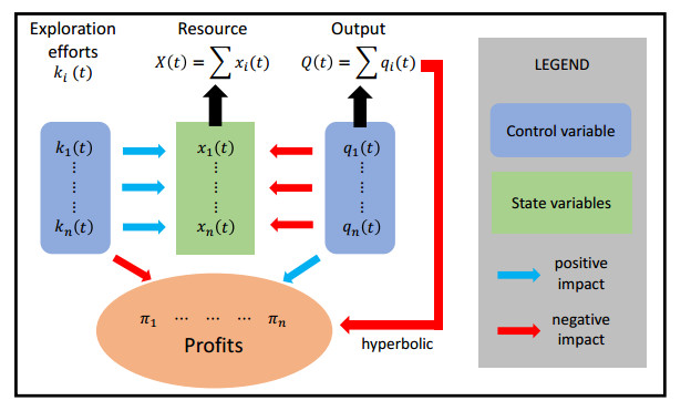
We consider a resource extraction model with the possibility of extending the resource stock by drilling efforts and an oligopolistic competition of symmetric firms. Assuming a hyperbolic market demand, we adopt the open-loop Nash equilibrium to analyze and compare the outcomes of a private vs a common resource pool. For both cases, the drilling efforts of the individual firms strongly depend on the market structure. For a low competition, the efforts increase the number of firms, and the opposite is true for a high competition. On the other hand, aggregate drilling efforts are different among the two types of pools and are opposite to Schumpeterian's hypothesis (i.e., they are either an inverted U-shaped (private pools) or strictly increasing (single pools)).

References

[1]	Aghion P, Akcigit U, Howitt P (2015) The Schumpeterian growth paradigm. Annu Rev Econ 7: 557–575. https://doi.org/10.1146/annurev-economics-080614-115412 doi: 10.1146/annurev-economics-080614-115412
[2]	Aghion P, Bloom N, Blundell R, et al. (2005) Competition and innovation: An inverted-U relationship. Q J Econ 120: 701–728. https://doi.org/10.1162/0033553053970214 doi: 10.1162/0033553053970214
[3]	Arrow K (1962) Economic welfare and the allocation of resources for invention. in R. Nelson (ed.), The Rate and Direction of Inventive Activity, Princeton, Princeton University Press. https://doi.org/10.1515/9781400879762-024
[4]	Arrow KJ, Chang S (1982) Optimal pricing, use, and exploration of uncertain resource stocks. J Environ Econ Manag 9: 1–10. https://doi.org/10.1016/0095-0696(82)90002-X doi: 10.1016/0095-0696(82)90002-X
[5]	Boyce J, Vojtassak L (2008) An 'Oil'igopoly theory of exploration. Resour Energy Econo 30: 428–454. https://doi.org/10.1016/j.reseneeco.2007.10.001 doi: 10.1016/j.reseneeco.2007.10.001
[6]	Cairns RD, Quyen NV (1998) Optimal exploration for and exploitation of heterogeneous mineral deposits. J Environ Econ Manag 35: 164–189. https://doi.org/10.1006/jeem.1998.1027 doi: 10.1006/jeem.1998.1027
[7]	Cellini R, Lambertini L (2002) A differential game approach to investment in product differentiation. J Econ Dyn Control 27: 51–62. https://doi.org/10.1016/S0165-1889(01)00026-4 doi: 10.1016/S0165-1889(01)00026-4
[8]	Dasgupta P, Gilbert R, Stiglitz J (1983) Strategic considerations in invention and innovation: The case of natural resources. Econometrica 51: 1439–1448. https://doi.org/10.2307/1912283 doi: 10.2307/1912283
[9]	Davison R (1978) Optimal depletion of an exhaustible resource with research and development towards an alternative technology. Rev Econ Stud 45: 335–367. https://doi.org/10.2307/2297350 doi: 10.2307/2297350
[10]	Delbono F, Lambertini L (2022) Innovation and product market concentration: Schumpeter, Arrow and the inverted-U Shape curve. Oxford Econ Pap 74: 297–311. https://doi.org/10.1093/oep/gpaa044 doi: 10.1093/oep/gpaa044
[11]	Deshmuk SD, Pliska SR (1980) Optimal consumption and exploration of nonrenewable resources under uncertainty. Econometrica 48: 177–200. https://doi.org/10.2307/1912024 doi: 10.2307/1912024
[12]	Dixit AK (1986) Comparative statics for oligopoly. Int Econ Rev 27: 103–122. https://doi.org/10.2307/2526609 doi: 10.2307/2526609
[13]	Feichtinger G, Hartl RF, Kort PM, et al. (2022) Asymmetric information in a capital accumulation differential game with spillover and learning effects. J Optimiz Theory Appl 194: 878–895. https://doi.org/10.1007/s10957-022-02054-7 doi: 10.1007/s10957-022-02054-7
[14]	Gilbert R (2006) Looking for Mr Schumpeter: Where are we in the competition-innovation debate?. in J. Lerner and S. Stern (eds), Innov Policy Econ NBER, MIT Press. https://doi.org/10.1086/ipe.6.25056183
[15]	Harris C, Vickers J (1995) Innovation and natural resources: A dynamic game with uncertainty. RAND J Econ 26: 418–430. https://doi.org/10.2307/2555996 doi: 10.2307/2555996
[16]	Hausman JA (1981) Exact consumer's surplus and deadweight loss Am Econ Rev 71: 662–476.
[17]	Hoel M (1978) Resource extraction, substitute production, and monopoly. J Econ Theory 19: 28–77. https://doi.org/10.1016/0022-0531(78)90053-4 doi: 10.1016/0022-0531(78)90053-4
[18]	Hoel M (1983) Monopoly resource extractions under the presence of predetermined substitute production. J Econ Theory 30: 201–212. https://doi.org/10.1016/0022-0531(83)90102-3 doi: 10.1016/0022-0531(83)90102-3
[19]	Lambertini L (2010) Oligopoly with hyperbolic demand: A differential game approach. J Optimiz Theory Appl 145: 108–119. https://doi.org/10.1007/s10957-009-9627-z doi: 10.1007/s10957-009-9627-z
[20]	Lambertini L (2013) Oligopoly, the Environment and Natural Resources, London, Routledge.
[21]	Lambertini L (2014) Exploration for nonrenewable resources in a dynamic oligopoly: An Arrovian result. Int Game Theory Rev 16: 1–11. https://doi.org/10.2139/ssrn.2197196 doi: 10.2139/ssrn.2197196
[22]	Loury G (1986) A Theory of 'Oil'igopoly: Cournot equilibrium in exhaustible resource market with fixed supplies. Int Econ Rev 27: 285–301. https://doi.org/10.2307/2526505 doi: 10.2307/2526505
[23]	Mohr E (1988) Appropriation of common access natural resources through exploration: The relevance of the open-loop concept. Int Econ Rev 29: 307–320. https://doi.org/10.2307/2526668 doi: 10.2307/2526668
[24]	Olsen TE (1988) Strategic considerations in invention and innovation: The case of natural resources revisited. Econometrica 56: 841–849. https://doi.org/10.2307/1912701 doi: 10.2307/1912701
[25]	Peterson FM (1978) A model of mining and exploration for exhaustible resources. J Environ Stud Manag 5: 236–251. https://doi.org/10.1016/0095-0696(78)90011-6 doi: 10.1016/0095-0696(78)90011-6
[26]	Polasky S (1992) Do oil firms act as 'Oil'igopolists? J Environ Econ Manag 23: 216–247. https://doi.org/10.1016/0095-0696(92)90002-E doi: 10.1016/0095-0696(92)90002-E
[27]	Polasky S (1996) Exploration and extraction in a duopoly-exhaustible resource market. Can J Econ 29: 473–492. https://doi.org/10.2307/136300 doi: 10.2307/136300
[28]	Quyen NV (1988) The optimal depletion and exploration of a nonrenewable resource. Econometrica 56: 1467–1471.
[29]	Quyen NV (1991) Exhaustible resources: A theory of exploration. Rev Econ Stud 58: 777–789. https://doi.org/10.2307/2297832 doi: 10.2307/2297832
[30]	Reinganum J, Stokey N (1985) Oligopoly extraction of a common property resource: The importance of the period of commitment in dynamic games. Int Econ Rev 26: 161–173. https://doi.org/10.2307/2526532 doi: 10.2307/2526532
[31]	Reynolds SS (1987) Capacity investment, preemption and commitment in an infinite horizon model. Int Econ Rev 28: 69–88. https://doi.org/10.2307/2526860 doi: 10.2307/2526860
[32]	Salant S (1976) Exhaustible resources and industrial structure: A Nash-Cournot approach to the world oil market. J Polit Econ 84: 1079–1094. https://doi.org/10.1086/260497 doi: 10.1086/260497
[33]	Schumpeter JA (1942) Capitalism, Socialism and Democracy, New York, Harper.
[34]	Tirole J (1988) The Theory of Industrial Organization, Cambridge, Mass, MIT Press.
[35]	Varian HR (1982) The nonparametric approach to demand analysis.. Econometrica 50: 945–973. https://doi.org/10.2307/1912771 doi: 10.2307/1912771

Reader Comments

Your name:*

Email:*
© 2024 the Author(s), licensee AIMS Press. This is an open access article distributed under the terms of the Creative Commons Attribution License (http://creativecommons.org/licenses/by/4.0)