Long-term economic impacts of coastal floods in Europe: a probabilistic analysis

Ignazio Mongelli; Michalis Vousdoukas; Luc Feyen; Antonio Soria; Juan-Carlos Ciscar; Ignazio Mongelli; Michalis Vousdoukas; Luc Feyen; Antonio Soria; Juan-Carlos Ciscar

doi:10.3934/environsci.2023033

AIMS Environmental Science

2023, Volume 10, Issue 5: 593-608. doi: 10.3934/environsci.2023033

Previous Article Next Article

Research article Special Issues

Long-term economic impacts of coastal floods in Europe: a probabilistic analysis

EU Commission - Joint Research Centre; Unit C6 - Economics of Climate Change, Energy and Transport, Sevilla, Spain

Received: 10 July 2023 Revised: 12 September 2023 Accepted: 25 September 2023 Published: 20 October 2023

In this article we quantify the long-term economic impacts of coastal flooding in Europe. In particular, how the direct coastal damages generate long-term economic losses that propagate and compound throughout the century. A set of probabilistic projections of inundation-related direct damages (to residential buildings, firms' physical assets and agriculture production) is used as an exogenous shock to a dynamic stochastic economic model. The article considers explicitly the uncertainty related to the economic agents' behaviour and other relevant macroeconomic assumptions, i.e., how would consumers finance the repairing of their homes, how long does it take for a firm to reconstruct, whether firms decide to build-back-better after the inundation and possibly compensate the losses with a productivity gain. Our findings indicate that the long-term impacts of coastal floods could be larger than the direct damages. Under a high emission scenario (RCP8.5) the EU27 plus UK could lose every year between 0.25% and 0.91% of output by 2100, twice as much as the direct damages. The welfare losses present a strong regional variation, with the South (Bulgaria, Greece, Italy, Malta, Portugal and Spain), and United Kingdom (UK) plus Ireland regions showing the highest damages and a significant part of the population that could suffer significant welfare losses by the end of the century.
- climate change,
- coastal impacts,
- uncertainty,
- economic analysis
Citation: Ignazio Mongelli, Michalis Vousdoukas, Luc Feyen, Antonio Soria, Juan-Carlos Ciscar. Long-term economic impacts of coastal floods in Europe: a probabilistic analysis[J]. AIMS Environmental Science, 2023, 10(5): 593-608. doi: 10.3934/environsci.2023033

Related Papers:

Abstract

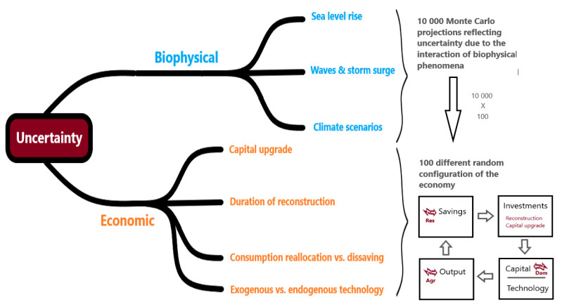
In this article we quantify the long-term economic impacts of coastal flooding in Europe. In particular, how the direct coastal damages generate long-term economic losses that propagate and compound throughout the century. A set of probabilistic projections of inundation-related direct damages (to residential buildings, firms' physical assets and agriculture production) is used as an exogenous shock to a dynamic stochastic economic model. The article considers explicitly the uncertainty related to the economic agents' behaviour and other relevant macroeconomic assumptions, i.e., how would consumers finance the repairing of their homes, how long does it take for a firm to reconstruct, whether firms decide to build-back-better after the inundation and possibly compensate the losses with a productivity gain. Our findings indicate that the long-term impacts of coastal floods could be larger than the direct damages. Under a high emission scenario (RCP8.5) the EU27 plus UK could lose every year between 0.25% and 0.91% of output by 2100, twice as much as the direct damages. The welfare losses present a strong regional variation, with the South (Bulgaria, Greece, Italy, Malta, Portugal and Spain), and United Kingdom (UK) plus Ireland regions showing the highest damages and a significant part of the population that could suffer significant welfare losses by the end of the century.

References

[1]	Vousdoukas M I, Mentaschi L, Voukouvalas E, et al. 2017. Extreme sea levels on the rise along Europe’s coasts. Earth’s Future 5: 304–323. https://doi.org/10.1002/2016EF000505 doi: 10.1002/2016EF000505
[2]	Godlewski G, Caporalini L, Deuss B. 2020. “Acqua Alta” and the need for the Mo.S.E. project, TU Delft, student research project report, available at: http://resolver.tudelft.nl/uuid:ea34a719-79c1-4c6e-b886-e0d92407bc9d (last access: 20 September 2022).
[3]	Botzen WJW, Deschenes O, Sanders M 2019. The Economic Impacts of Natural Disasters: A Review of Models and Empirical Studies. Rev Environ Econ Policy 13: 167–188. https://doi.org/10.1093/reep/rez004 doi: 10.1093/reep/rez004
[4]	Bosello F, Nicholls RJ, Richards J, et al. (2012) Economic impacts of climate change in Europe: sea level rise. Clim Change 112: 63–81. https://doi.org/10.1007/s10584-011-0340-1 doi: 10.1007/s10584-011-0340-1
[5]	Nishiura O, Tamura M, Fujimori S, et al. (2020). An Assessment of Global Macroeconomic Impacts Caused by Sea Level Rise Using the Framework of Shared Socioeconomic Pathways and Representative Concentration Pathways. Sustainability 12: 3737. https://doi.org/10.3390/su12093737 doi: 10.3390/su12093737
[6]	Schinko T, Drouet L, Vrontisi Z, et al. 2020. Economy-wide effects of coastal flooding due to sea level rise: a multi-model simultaneous treatment of mitigation, adaptation, and residual impacts. Environ. Commun 2: 015002. https://doi.org/10.1088/2515-7620/ab6368
[7]	Dottori F, Szewczyk W, Ciscar J-C, et al. 2018. Increased human and economic losses from river flooding with anthropogenic warming. Nat Clim Change 8: 781–786. https://doi.org/10.1038/s41558-018-0257-z doi: 10.1038/s41558-018-0257-z
[8]	Tanoue M, Taguchi R, Nakata S, et al. 2020. Estimation of direct and indirect economic losses caused by a flood with long-lasting inundation: Application to the 2011 Thailand flood. Water Resour Res 56. https://doi.org/10.1029/2019WR026092
[9]	Mochizuki J, Mechler R, Hochrainer-Stigler S, et al. 2014. Revisiting the ‘disaster and development’ debate–Toward a broader understanding of macroeconomic risk and resilience. Clim Risk Manag 3: 39–54. https://doi.org/10.1016/j.crm.2014.05.002 doi: 10.1016/j.crm.2014.05.002
[10]	Naqvi A, Monasterolo I 2021. Assessing the cascading impacts of natural disasters in a multi-layer behavioral network framework. Sci Rep 11: 20146. https://doi.org/10.1038/s41598-021-99343-4 doi: 10.1038/s41598-021-99343-4
[11]	Duan H, Mo J, Fan Y, et al. 2018. Achieving China's energy and climate policy targets in 2030 under multiple uncertainties. En Econ 70: 45–60. https://doi.org/10.1016/j.eneco.2017.12.022 doi: 10.1016/j.eneco.2017.12.022
[12]	Zhang S, Chen W 2022. Assessing the energy transition in China towards carbon neutrality with a probabilistic framework. Nat Commun 13: 87. https://doi.org/10.1038/s41467-021-27671-0 doi: 10.1038/s41467-021-27671-0
[13]	Vousdoukas MI, Mentaschi L, Hinkel J, et al. 2020. Economic motivation for raising coastal flood defenses in Europe. Nat Commun 11: 2119. https://doi.org/10.1038/s41467-020-15665-3 doi: 10.1038/s41467-020-15665-3
[14]	Kirezci E, Young IR, Ranasinghe R, et al. 2020. Projections of global-scale extreme sea levels and resulting episodic coastal flooding over the 21st Century. Scientific Reports 10: 11629. https://doi.org/10.1038/s41598-020-67736-6 doi: 10.1038/s41598-020-67736-6
[15]	Tsigaris P, Wood J 2016. A simple climate-Solow model for introducing the economics of climate change to undergraduate students. Int Rev Econ 23: 65–81. https://doi.org/10.1016/j.iree.2016.06.002 doi: 10.1016/j.iree.2016.06.002
[16]	Depsky N, Bolliger I, Allen D, et al. 2023. DSCIM-Coastal v1.1: an open-source modeling platform for global impacts of sea level rise, Geosci Model Dev 16: 4331–4366. https://doi.org/10.5194/gmd-16-4331-2023 doi: 10.5194/gmd-16-4331-2023
[17]	Fankhauser S, Tol RS 2005. On climate change and economic growth. Resource and Energy Econ 27: 1–17. https://doi.org/10.1016/j.reseneeco.2004.03.003 doi: 10.1016/j.reseneeco.2004.03.003
[18]	Dietz S, Stern N (2015) Endogenous Growth, Convexity of Damage and Climate Risk: How Nordhaus' Framework Supports Deep Cuts in Carbon Emissions. Econ J 120: 574 –620. https://doi.org/10.1111/ecoj.12188 doi: 10.1111/ecoj.12188
[19]	Bosello F, De Cian E (2014) Climate change, sea level rise, and coastal disasters. A review of modelling practices. Energy Econ 46: 593–605. https://doi.org/10.1016/j.eneco.2013.09.002
[20]	Piontek F, Kalkuhl M, Kriegler E, et al. 2019. Economic Growth Effects of Alternative Climate Change Impact Channels in Economic Modeling. Environ Resour Econ 73: 1357–1385. https://doi.org/10.1007/s10640-018-00306-7 doi: 10.1007/s10640-018-00306-7
[21]	DG Ecfin (2021) The 2021 Ageing Report Economic & Budgetary Projections for the EU Member States (2019–2070). Institutional paper 148. Brussels.
[22]	Solow R M (1956). A contribution to the theory of economic growth. The quarterly journal of economics 70: 65–94. https://doi.org/10.2307/1884513 doi: 10.2307/1884513
[23]	Verschuur J, Koks E E, Haque A, et al. (2020) Prioritising resilience policies to reduce welfare losses from natural disasters: a case study for coastal Bangladesh. Glob Environ Change 65: 102179. https://doi.org/10.1016/j.gloenvcha.2020.102179 doi: 10.1016/j.gloenvcha.2020.102179
[24]	Walsh B, Hallegatte S (2020) Measuring Natural Risks in the Philippines: Socioeconomic Resilience and Wellbeing Losses. Econ Disaster Clim Chang 4: 249–293. https://doi.org/10.1007/s41885-019-00047-x doi: 10.1007/s41885-019-00047-x
[25]	Feyen L, Ciscar JC, Gosling S, et al. (2020) Climate change impacts and adaptation in Europe. JRC PESETA IV final report. EUR 30180EN, Publications Office of the European Union, Luxembourg, ISBN 978-92-76-18123-1, doi: 10.2760/171121,JRC119178.
[26]	Kesten H (1971) S ome nonlinear stochastic growth models. Bull New Ser Am Math Soc 77: 492–511. https://doi.org/10.1090/S0002-9904-1971-12732-5 doi: 10.1090/S0002-9904-1971-12732-5
[27]	Schenk-Hoppé K R, Schmalfuss B (2001) Random fixed points in a stochastic Solow growth model. J Math Econ 36: 19–30. https://doi.org/10.1016/S0304-4068(01)00062-3 doi: 10.1016/S0304-4068(01)00062-3
[28]	Feicht R, Stummer W (2010) Complete closed-form solution to a stochastic growth model and corresponding speed of economic recovery (No. 05/2010). IWQW Discussion Papers.
[29]	Hallegatte S, Dumas P (2009) Can natural disasters have positive consequences? Investigating the role of embodied technical change. Ecological Econ 68: 777–786. https://doi.org/10.1016/j.ecolecon.2008.06.011 doi: 10.1016/j.ecolecon.2008.06.011
[30]	Skidmore M, Toya H (2002) Do natural disasters promote long-run growth? Econ Inq 40: 664–687. https://doi.org/10.1093/ei/40.4.664 doi: 10.1093/ei/40.4.664
[31]	Albala-Bertrand JM (1993) Political Economy of Large Natural Disasters: With Special Reference to Developing Countries. OUP Catalogue, Oxford University Press, number 9780198287650.
[32]	Crespo CJ, Hlouskova J, Obersteiner M (2008) Natural disasters as creative destruction? Evidence from developing countries. Econ Inq 46: 214–226. https://doi.org/10.1111/j.1465-7295.2007.00063.x doi: 10.1111/j.1465-7295.2007.00063.x
[33]	Hallegatte S, Hourcade JC, Dumas P (2007) Why economic dynamics matter in assessing climate change damages: Illustration on extreme events. Ecological Econ 62: 330–340. https://doi.org/10.1016/j.ecolecon.2006.06.006 doi: 10.1016/j.ecolecon.2006.06.006
[34]	Benson C, Clay E (2004) Understanding the economic and financial impact of natural disasters. The International Bank for Reconstruction and Development. The World Bank, Washington D.C.Supplementary information https://doi.org/10.1596/0-8213-5685-2
[35]	Zhou Z, Zhang L (2021) Destructive destruction or creative destruction? Unravelling the effects of tropical cyclones on economic growth. Econ Anal Policy 70: 380–393. https://doi.org/10.1016/j.eap.2021.03.010 doi: 10.1016/j.eap.2021.03.010
[36]	Panwar V, Sen S (2019) Economic impact of natural disasters: An empirical re-examination. Margin J Appl Econ Res 13: 109–139. https://doi.org/10.1177/0973801018800087 doi: 10.1177/0973801018800087
[37]	Cavallo E, Galiani S, Noy I, et al. (2013) Catastrophic Natural Disasters and Economic Growth. Rev Econ Stat 95: 1549–1561. https://doi.org/10.1162/REST_a_00413 doi: 10.1162/REST_a_00413
[38]	Hornbeck R, Keniston D (2017) Creative Destruction: Barriers to Urban Growth and the Great Boston Fire of 1872. Am Econ Rev 107: 1365–1398. https://doi.org/10.1257/aer.20141707 doi: 10.1257/aer.20141707
[39]	Carpenter O, Platt S, Mahdavian F (2018) Disaster Recovery Case Studies: UK Floods 2007. Cambridge Centre for Risk Studies at the University of Cambridge Judge Business School.
[40]	Kumar S, Russell R R (2002) Technological change, technological catch-up, and capital deepening: relative contributions to growth and convergence. Am Econ Rev 92: 527–548. https://doi.org/10.1257/00028280260136381 doi: 10.1257/00028280260136381
[41]	Arrow KJ (1962) The economic implications of learning by doing. Rev Econ Stud 29: 155–173. https://doi.org/10.2307/2295952 doi: 10.2307/2295952
[42]	Romer PM (1986) Increasing returns and long-run growth. J Polit Econ 94: 1002–1037. https://doi.org/10.1086/261420 doi: 10.1086/261420
[43]	Howitt P (2005) Health, human capital and economic growth: a Schumpeterian perspective. In: Health and Economic Growth: Findings and Policy Implications, ed. G. Lopez- Casasnovas. B. Rivera, and L. Currais. Cambridge. MA: MIT Press https://doi.org/10.7551/mitpress/3451.003.0005
[44]	Feenstra RC, Inklaar R, Timmer MP (2015) The Next Generation of the Penn World Table. Am Econ Rev 105: 3150–3182. ttps://doi.org/10.1257/aer.20130954 doi: 10.1257/aer.20130954
[45]	European Commission–Eurostat, 2021. Annual sector accounts - Non-financial transactions (nasa_10_nf_tr).
[46]	The World Bank, World Development Indicators, 2021. Gross savings (% of GDP). World Bank national accounts data, and OECD National Accounts data files. Retrieved from https://data.worldbank.org/indicator/NY.GNS.ICTR.ZS
[47]	Mastrandrea, M.D., Field, C.B., Stocker, T.F., Edenhofer, O., Ebi, K.L., Frame, D.J., Held, H., Kriegler, E., Mach, K.J., Matschoss, P.R., Plattner, G.-K., Yohe, G.W. and Zwiers, F.W., 2010. Guidance Note for Lead Authors of the IPCC Fifth Assessment Report on Consistent Treatment of Uncertainties. Intergovernmental Panel on Climate Change (IPCC). Available at http://www.ipcc.ch

Environ-10-05-033-s001.pdf

Reader Comments

Your name:*

Email:*
© 2023 the Author(s), licensee AIMS Press. This is an open access article distributed under the terms of the Creative Commons Attribution License (http://creativecommons.org/licenses/by/4.0)