The occurrence of defects in solar cells is intrinsically related to a reduction in the efficiency and reliability of these devices. Therefore, monitoring techniques, such as lock-in thermography, electroluminescence and the I-V characteristic curve are adopted in order to evaluate the integrity of the solar cells. In the present work, a novel experimental procedure for the lock-in thermography of solar cells is proposed, aiming to improve the detection capability of the assay. Conventional techniques use pulse width modulation to operate the cell at a fixed point on the I-V curve. Instead, we propose a methodology based on a sinusoidal electric current excitation in order to extend the range of operational points that are close to the maximum power point as the cell operates in the field. Some traditional image processing techniques (principal component analysis, the fast Fourier transform and the four-step phase-shifting method) have been used to analyze the thermal images captured by an infrared camera during steady-state operation mode of the solar cells using both sinusoidal electric current signal and standard pulse width modulation procedures. Comparison between the results of both procedures found that this novel approach provides smoother and clearer delimitation of the defects. Furthermore, the contrast of the phase images was found to exhibit significant changes between the defective and non-defective regions for different modulation frequencies and types of defects. From the achieved results, it was possible to obtain a satisfactory characterization of the existing defects.
Citation: Thiago M. Vieira, Ézio C. Santana, Luiz F. S. Souza, Renan O. Silva, Tarso V. Ferreira, Douglas B. Riffel. A novel experimental procedure for lock-in thermography on solar cells[J]. AIMS Energy, 2023, 11(3): 503-521. doi: 10.3934/energy.2023026
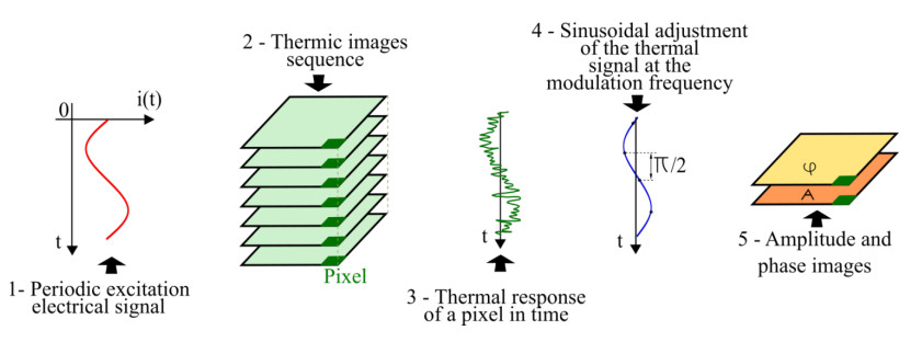
The occurrence of defects in solar cells is intrinsically related to a reduction in the efficiency and reliability of these devices. Therefore, monitoring techniques, such as lock-in thermography, electroluminescence and the I-V characteristic curve are adopted in order to evaluate the integrity of the solar cells. In the present work, a novel experimental procedure for the lock-in thermography of solar cells is proposed, aiming to improve the detection capability of the assay. Conventional techniques use pulse width modulation to operate the cell at a fixed point on the I-V curve. Instead, we propose a methodology based on a sinusoidal electric current excitation in order to extend the range of operational points that are close to the maximum power point as the cell operates in the field. Some traditional image processing techniques (principal component analysis, the fast Fourier transform and the four-step phase-shifting method) have been used to analyze the thermal images captured by an infrared camera during steady-state operation mode of the solar cells using both sinusoidal electric current signal and standard pulse width modulation procedures. Comparison between the results of both procedures found that this novel approach provides smoother and clearer delimitation of the defects. Furthermore, the contrast of the phase images was found to exhibit significant changes between the defective and non-defective regions for different modulation frequencies and types of defects. From the achieved results, it was possible to obtain a satisfactory characterization of the existing defects.

| [1] | Pinho J, Galdino M (2014) Engineering manual for photovoltaic systems. CEPEL—CRESESB. Available from: http://www.cresesb.cepel.br/publicacoes/download/Manual_de_Engenharia_FV_2014.pdf. |
| [2] |
Olarte J, Dauvergne JL, Herrán A, et al. (2019) Validation of thermal imaging as a tool for failure mode detection development. AIMS Energy 7: 646–659. https://doi.org/10.3934/energy.2019.5.646 doi: 10.3934/energy.2019.5.646

|
| [3] | Breintenstein O, Langenkamp M (2010) Lock-in Thermography—Basics and use for evaluating electronic devices and materials. Berlin, Springer. https://doi.org/10.1007/978-3-642-02417-7 |
| [4] |
Da Silva WF, Melo RAC, Grosso M, et al. (2020) Active thermography data-processing algorithm for nondestructive testing of materials. IEEE Access 8: 175054–175062. https://doi.org/10.1109/ACCESS.2020.3025329 doi: 10.1109/ACCESS.2020.3025329
|
| [5] |
Rösch R, Tanenbaum DM, Jørgensen M, et al. (2012) Investigation of the degradation mechanisms of a variety of organic photovoltaic devices by combination of imaging techniques—The ISOS-3 inter-laboratory collaboration. Energy Environ Sci 5: 6521–6540. https://doi.org/10.1039/c2ee03508a doi: 10.1039/c2ee03508a
|
| [6] |
Pletzer TM, van Mölken JI, Rißand S, et al. (2015) Influence of cracks on the local current-voltage parameters of silicon solar cells. Prog Photovoltaics: Res Appl 23: 428–436. https://doi.org/10.1002/pip.2443 doi: 10.1002/pip.2443
|
| [7] |
Hoppe H, Bachmann J, Muhsin B, et al. (2010) Quality control of polymer solar modules by lock-in thermography. J Appl Phys, 107. https://doi.org/10.1063/1.3272709 doi: 10.1063/1.3272709
|
| [8] |
Breitenstein O, Bauer J, Bothe K, et al. (2011) Can luminescence imaging replace lock-in thermography on solar cells? IEEE J Photovoltaic 1: 159–167. https://doi.org/10.1109/JPHOTOV.2011.2169394 doi: 10.1109/JPHOTOV.2011.2169394
|
| [9] |
Breitenstein O, Rakotoniaina JP, al Rifai MH (2003) Quantitative evaluation of shunts in solar cells by lock-in thermography. Prog Photovoltaics: Res Appl 11: 515–526. https://doi.org/10.1002/pip.520 doi: 10.1002/pip.520
|
| [10] |
Peloso MP, Meng L, Bhatia CS (2015) Combined thermography and luminescence imaging to characterize the spatial performance of multicrystalline si wafer solar cells. IEEE J Photovoltaic 5: 102–111. https://doi.org/10.1109/JPHOTOV.2014.2362303 doi: 10.1109/JPHOTOV.2014.2362303
|
| [11] |
Hepp J, Machui F, Egelhaaf HJ, et al. (2016) Automatized analysis of IR-images of photovoltaic modules and its use for quality control of solar cells. Energy Sci Eng 4: 363–371. https://doi.org/10.1002/ese3.140 doi: 10.1002/ese3.140
|
| [12] |
Asadpour R, Sulas-Kern DB, Johnston S, et al. (2020) Dark lock-in thermography identifies solder bond failure as the root cause of series resistance increase in fielded solar modules. IEEE J Photovoltaic 10: 1409–1416. https://doi.org/10.1109/JPHOTOV.2020.3003781 doi: 10.1109/JPHOTOV.2020.3003781
|
| [13] |
Breitenstein O, Sturm S (2019) Lock-in thermography for analyzing solar cells and failure analysis in other electronic components. Quant InfraRed Thermogr J 16: 1–15. https://doi.org/10.1080/17686733.2018.1563349 doi: 10.1080/17686733.2018.1563349
|
| [14] |
Breitenstein O (2013) Illuminated versus dark lock-in thermography investigations of solar cells. Int J Nanopart, 6. https://doi.org/10.1504/IJNP.2013.054983 doi: 10.1504/IJNP.2013.054983
|
| [15] |
Dahlberg P, Ziegeler NJ, Nolte PW, et al. (2022) Design and construction of an LED-Based excitation source for lock-in thermography. Appl Sci 12: 2940. https://doi.org/10.3390/app12062940. doi: 10.3390/app12062940
|
| [16] |
He Y, Du B, Huang S (2018) Noncontact electromagnetic induction excited infrared thermography for photovoltaic cells and modules inspection. IEEE Trans Ind Informatics 14: 5585–5593. https://doi.org/10.1109/TII.2018.2822272 doi: 10.1109/TII.2018.2822272
|
| [17] | Halwachs M (2014) Development of a dark lock-in thermography (DLIT) system and its application for characterizing thin film and crystalline photovoltaic generators (Doctoral dissertation). https://doi.org/10.34726/hss.2014.24877 |
| [18] |
Shrestha R, Park J, Kim W (2016) Application of thermal wave imaging and phase shifting method for defect detection in stainless steel. Infrared Phys Technol 76: 676–683. https://doi.org/10.1016/j.infrared.2016.04.033 doi: 10.1016/j.infrared.2016.04.033
|
| [19] |
Hongyu K, Sandanielo VLM, Oliveira Junior GJ (2016) Principal components analysis: theoretical summary, application and interpretation. ES Eng Sci 5: 83–90. https://doi.org/10.18607/ES201653398 doi: 10.18607/ES201653398
|
| [20] | N. L. J. (1959) Review of An Introduction to Multivariate Statistical Analysis; Some Aspects of Multivariate Analysis, by T. W. Anderson & S. N. Roy. 9: 67-68. Inc Stat https://doi.org/10.2307/2986618 |
| [21] |
Ibarra-Castanedo C, Tarpani J, Maldague X (2013) Nondestructive testing with thermography. Eur J Phys, 34. https://doi.org/10.1088/0143-0807/34/6/S91 doi: 10.1088/0143-0807/34/6/S91
|
| [22] | Krapez JC (1998) Compared performances of four algorithms used for modulation thermography. QIRT'98 Quantitative Infrared Thermography. Lodz, Poland. https://doi.org/10.21611/qirt.1998.023 |
| [23] | Gonzalez RC, Wood RC (2018) Digital Image Processing. 4a ed. Pearson. Available from: https://www.pearson.com/en-us/subject-catalog/p/digital-image-processing/P200000003224. |
| [24] | Strang G (1994) Wavelets. American Scientist 82: 250–255, JSTOR. Available from: https://www.jstor.org/stable/29775194?seq = 1. |
| [25] | Macedo MS (2022) Classification of hydrophobicity in electrical insulators using frequency analysis and ANN. Masters dissertation, Federal University of Sergipe. São Cristóvão. Available from: http://ri.ufs.br/jspui/handle/riufs/16894. |
| [26] | Brazilian Association of Technical Standards (2021) NBR—16969: 2021, Non-destructive testing—Infrared Thermography—General Principles. Rio de Janeiro. Available from: https://www.gedweb.com.br/aplicacao/usuario/asp/detalhe_nbr.asp?assinc = 1 & nbr = 13128. |
| [27] | Brazilian Association of Technical Standards (2013) NBR—15572: 2013, Non-destructive testing—Thermography—Guide for inspection of electrical and mechanical equipment. Rio de Janeiro. Available from: https://www.gedweb.com.br/aplicacao/usuario/asp/detalhe_nbr.asp?assinc = 1 & nbr = 27135. |
| [28] | International Electrotechnical Commission (2018) IEC 62446-1-Photovoltaic (PV) systems—Requirements for testing, documentation and maintenance—Part 1: Grid connected systems—Documentation, commissioning tests and inspection. IEC, Geneva, Switzerland. Available from: https://www.gedweb.com.br/aplicacao/usuario/asp/detalhe_nie.asp?assinc = 1 & nie = 106520. |
| [29] | International Electrotechnical Commission (2020) IEC 62446-2-Photovoltaic (PV) systems—Requirements for testing, documentation and maintenance—Part 1: Grid connected systems—Maintenance of PV systems. IEC, Geneva, Switzerland. Available from: https://webstore.iec.ch/publication/27382. |
| [30] | International Electrotechnical Commission (2017) IEC TS 62446-3-Photovoltaic (PV) systems—Requirements for testing, documentation and maintenance-Part 3: Photovoltaic modules and plants—Outdoor infrared thermography. IEC, Geneva, Switzerland. Available from: https://webstore.iec.ch/publication/28628. |


Figures(13) / Tables(2)

Thiago M. Vieira, Ézio C. Santana, Luiz F. S. Souza, Renan O. Silva, Tarso V. Ferreira, Douglas B. Riffel. A novel experimental procedure for lock-in thermography on solar cells[J]. AIMS Energy, 2023, 11(3): 503-521. doi: 10.3934/energy.2023026


 DownLoad: