Designing an energy management system for household consumptions with an off-grid hybrid power system

Mohamed Elweddad; Muhammet Güneşer; Ziyodulla Yusupov; Mohamed Elweddad; Muhammet Güneşer; Ziyodulla Yusupov

doi:10.3934/energy.2022036

AIMS Energy

2022, Volume 10, Issue 4: 801-830. doi: 10.3934/energy.2022036

Previous Article Next Article

Research article Topical Sections

Designing an energy management system for household consumptions with an off-grid hybrid power system

Department of Electrical and Electronic Engineering, Karabuk University, Karabuk, Turkey

Received: 06 March 2022 Revised: 13 June 2022 Accepted: 23 June 2022 Published: 15 July 2022

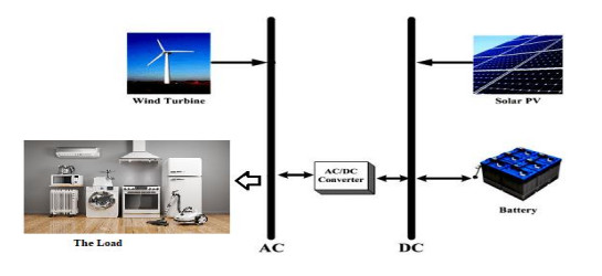
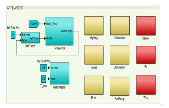
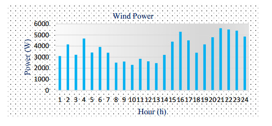
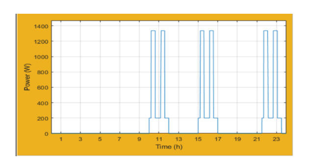
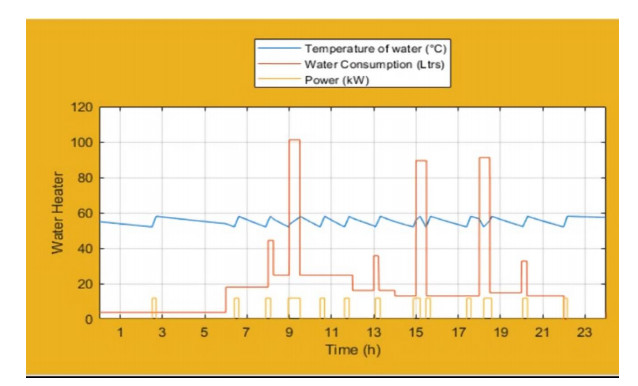
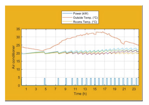
This paper analyzes the effect of meteorological variables such as solar irradiance and ambient temperature in addition to cultural factors such as consumer behavior levels on energy consumption in buildings. Reducing demand peaks to achieve a stable daily load and hence lowering electricity bills is the goal of this work. Renewable generation sources, including wind and Photovoltaics systems (PV) as well as battery storage are integrated to supply the managed home load. The simulation model was conducted using Matlab R2019b on a personal laptop with an Intel Core i7 with 16 GB memory. The model considered two seasonal scenarios (summer and winter) to account for the variable available energy sources and end-user electric demand which is classified into three demand periods, peak-demand, mid-demand, and low-demand, to evaluate the modeled supply-demand management strategy. The obtained results showed that the surrounding temperature and the number of family members significantly impact the rate of electricity consumption. The study was designed to optimize and manage electricity consumption in a building fed by a standalone hybrid energy system.
- home energy management,
- energy consumption modeling,
- hybrid system,
- smart loads,
- home appliances modeling
Citation: Mohamed Elweddad, Muhammet Güneşer, Ziyodulla Yusupov. Designing an energy management system for household consumptions with an off-grid hybrid power system[J]. AIMS Energy, 2022, 10(4): 801-830. doi: 10.3934/energy.2022036

Related Papers:

Abstract

This paper analyzes the effect of meteorological variables such as solar irradiance and ambient temperature in addition to cultural factors such as consumer behavior levels on energy consumption in buildings. Reducing demand peaks to achieve a stable daily load and hence lowering electricity bills is the goal of this work. Renewable generation sources, including wind and Photovoltaics systems (PV) as well as battery storage are integrated to supply the managed home load. The simulation model was conducted using Matlab R2019b on a personal laptop with an Intel Core i7 with 16 GB memory. The model considered two seasonal scenarios (summer and winter) to account for the variable available energy sources and end-user electric demand which is classified into three demand periods, peak-demand, mid-demand, and low-demand, to evaluate the modeled supply-demand management strategy. The obtained results showed that the surrounding temperature and the number of family members significantly impact the rate of electricity consumption. The study was designed to optimize and manage electricity consumption in a building fed by a standalone hybrid energy system.

References

[1]	Du P, Lu N (2011) Appliance commitment for household load scheduling. IEEE Trans Smart Grid 2: 411–419. https://doi.org/10.1109/TSG.2011.2140344 doi: 10.1109/TSG.2011.2140344
[2]	Mishra A, Irwin D, Shenoy P, et al. (2013) Greencharge: Managing renewable energy in smart buildings. IEEE J Selected Areas Commun 31: 1281–1293. https://doi.org/10.1109/JSAC.2013.130711 doi: 10.1109/JSAC.2013.130711
[3]	Li W, Logenthiran T, Woo WL (2015) Intelligent multi agent system for smart home energy management. IEEE Innovative Smart Grid Technologies Asia (ISGT ASIA), Bangkok, Thailand. https://doi.org/10.1109/ISGT-Asia.2015.7386985 doi: 10.1109/ISGT-Asia.2015.7386985
[4]	Corno F, Razzak F (2012) Intelligent energy optimization for user intelligible goals in smart home environments. IEEE Trans Smart Grid 3: 2128–2135. https://doi.org/10.1109/TSG.2012.2214407 doi: 10.1109/TSG.2012.2214407
[5]	Khan ZA, Ahmed S, Nawaz R, et al. (2015) Optimization based individual and cooperative DSM in smart grids: A review. Power Generation System and Renewable Energy Technologies (PGSRET), IEEE. https://doi.org/10.1109/PGSRET.2015.7312239 doi: 10.1109/PGSRET.2015.7312239
[6]	Boynuegri AR, Yagcitekin B, Baysal M, et al. (2013) Energy management algorithm for smart home with renewable energy sources. 4th International Conference on Power Engineering, Energy and Electrical Drives, IEEE, 1753–1758. https://doi.org/10.1109/PowerEng.2013.6635883
[7]	Saha A, Kuzlu M, Khamphanchai W, et al. (2014) A home energy management algorithm in a smart house integrated with renewable energy. IEEE PES Innovative Smart Grid Technologies, Europe, IEEE, 1–6. https://doi.org/10.1109/ISGTEurope.2014.7028970 doi: 10.1109/ISGTEurope.2014.7028970
[8]	Et-Tolba El H, Ouassaid, M, Maaroufi M (2016) Smart home appliances modeling and simulation for energy consumption profile development: Application to Moroccan real environment case study. In 2016 International Renewable and Sustainable Energy Conference (IRSEC), 1050–1055. https://ieeexplore.ieee.org/abstract/document/7983908
[9]	Schné T, Jaskó S, Simon G (2015) Dynamic models of a home refrigerator. MACRo 1: 103–112. https://doi.org/10.1515/macro-2015-0010 doi: 10.1515/macro-2015-0010
[10]	Shareef H, Ahmed MS, Mohamed A, et al. (2018) Review on home energy management system considering demand responses, smart technologies, and intelligent controllers. IEEE Access 6: 24498–24509. https://doi.org/10.1109/ACCESS.2018.2831917 doi: 10.1109/ACCESS.2018.2831917
[11]	Boodi A, Beddiar K, Benamour M, et al. (2018) Intelligent systems for building energy and occupant comfort optimization: A state of the art review and recommendations. Energies 11: 2604. https://doi.org/10.3390/en11102604 doi: 10.3390/en11102604
[12]	Zhang D, Evangelisti S, Lettieri P, et al. (2016) Economic and environmental scheduling of smart homes with microgrid: DER operation and electrical tasks. Energy Convers Manag 110: 113–124. https://doi.org/10.1016/j.enconman.2015.11.056 doi: 10.1016/j.enconman.2015.11.056
[13]	Naz M, Iqbal Z, Javaid N, et al. (2018) Efficient power scheduling in smart homes using hybrid grey wolf differential evolution optimization technique with real time and critical peak pricing schemes. Energies 11: 384. https://doi.org/10.3390/en11020384 doi: 10.3390/en11020384
[14]	Xiong G, Chen C, Kishore S, et al. (2011) Smart (in home) power scheduling for demand response on the smart grid. ISGT 2011, IEEE, 1–7. Available from: https://ieeexplore.ieee.org/abstract/document/5759154.
[15]	Radhakrishnan A, Selvan MP (2014) Load scheduling for smart energy management in residential buildings with renewable sources. In 2014 Eighteenth National Power Systems Conference (NPSC), 1–6. https://doi.org/10.1109/NPSC.2014.7103825 doi: 10.1109/NPSC.2014.7103825
[16]	Zhang Y, Zeng P, Li S, et al. (2015) A novel multiobjective optimization algorithm for home energy management system in smart grid. Math Probl Eng, 2015. https://doi.org/10.1155/2015/807527 doi: 10.1155/2015/807527
[17]	Fanti MP, Mangini AM, Roccotelli M (2018) A simulation and control model for building energy management. Control Eng Pract 72: 192–205. https://doi.org/10.1016/j.conengprac.2017.11.010 doi: 10.1016/j.conengprac.2017.11.010
[18]	dos Reis FB, Tonkoski R, Hansen TM (2020) Synthetic residential load models for smart city energy management simulations. IET Smart Grid 3: 342–354. https://doi.org/10.1049/iet-stg.2019.0296 doi: 10.1049/iet-stg.2019.0296
[19]	Hosseini A, Safari MM, Nazari heris M, et al. (2021) Application of Internet of Things (IoT) to demand side management in smart grids. In: Introduction to Internet of Things in Management Science and Operations Research, 169–183. Springer, Cham. https://doi.org/10.1007/978-3-030-74644-5_8
[20]	Tostado-Véliz M, Gurung S, Jurado F (2022) Efficient solution of many objective home energy management systems. Int J Electr Power Energy Syst 136: 107666. https://doi.org/10.1016/j.ijepes.2021.107666 doi: 10.1016/j.ijepes.2021.107666
[21]	Tostado-Véliz M, Mouassa S, Jurado F (2021) A MILP framework for electricity tariff choosing decision process in smart homes considering 'Happy Hours' tariffs. Int J Electr Power Energy Syst 131: 107139. https://doi.org/10.1016/j.ijepes.2021.107139 doi: 10.1016/j.ijepes.2021.107139
[22]	Tostado-Véliz M, Bayat M, Ghadimi A, et al. (2021) Home energy management in off grid dwellings: Exploiting flexibility of thermostatically controlled appliances. J Cleane Prod 310: 127507. https://doi.org/10.1016/j.jclepro.2021.127507 doi: 10.1016/j.jclepro.2021.127507
[23]	Tostado-Véliz M, Icaza-Alvarez D, Jurado F (2021) A novel methodology for optimal sizing photovoltaic-battery systems in smart homes considering grid outages and demand response. Renewable Energy 170: 884–896. https://doi.org/10.1016/j.renene.2021.02.006 doi: 10.1016/j.renene.2021.02.006
[24]	Molla T, Khan B, Moges B, et al. (2019) Integrated optimization of smart home appliances with cost-effective energy management system. CSEE J Power Energy Syst 5: 249–258. https://doi.org/10.17775/CSEEJPES.2019.00340 doi: 10.17775/CSEEJPES.2019.00340
[25]	Lee S, Choi DH (2020) Energy management of smart home with home appliances, energy storage system and electric vehicle: A hierarchical deep reinforcement learning approach. Sensors 20: 2157. https://doi.org/10.3390/s20072157 doi: 10.3390/s20072157
[26]	Waseem M, Lin Z, Liu S, et al. (2020) Optimal GWCSO-based home appliances scheduling for demand response considering end users comfort. Electr Power Syst Res 187: 106477. https://doi.org/10.1016/j.epsr.2020.106477 doi: 10.1016/j.epsr.2020.106477
[27]	Alimi OA, Ouahada K (2018) Smart home appliances scheduling to manage energy usage. 2018 IEEE 7th International Conference on Adaptive Science & Technology (ICAST), IEEE. https://doi.org/10.1109/ICASTECH.2018.8507138 doi: 10.1109/ICASTECH.2018.8507138
[28]	Mahmood A, Javaid N, Khan NA, et al. (2016) An optimized approach for home appliances scheduling in smart grid. In 2016 19th International Multi Topic Conference (INMIC), 1–5. https://doi.org/10.1109/INMIC.2016.7840158 doi: 10.1109/INMIC.2016.7840158
[29]	Amer A, Shaban K, Gaouda, et al. (2021) Home energy management system embedded with a multi-objective demand response optimization model to benefit customers and operators. Energies 14: 257. https://doi.org/10.3390/en14020257 doi: 10.3390/en14020257
[30]	Minhas DM, Frey G (2019) Modeling and optimizing energy supply and demand in home area power network (HAPN). IEEE Access 8: 2052–2072. https://doi.org/10.1109/ACCESS.2019.2962660 doi: 10.1109/ACCESS.2019.2962660
[31]	Soleimani H, Chhetri P, Fathollahi-Fard A, et al. (2022) Sustainable closed-loop supply chain with energy efficiency: Lagrangian relaxation, reformulations and heuristics. Ann Oper Res: 1–26. https://doi.org/10.1007/s10479-022-04661-z doi: 10.1007/s10479-022-04661-z
[32]	Ghadami N, Gheibi M, Kian Z, et al. (2021) Implementation of solar energy in smart cities using an integration of artificial neural network, photovoltaic system and classical Delphi methods. Sustain. Cities Soc 74: 103149. https://doi.org/10.1016/j.scs.2021.103149 doi: 10.1016/j.scs.2021.103149
[33]	Shahsavar M, Akrami M, Gheibi M, et al. (2021) Constructing a smart framework for supplying the biogas energy in green buildings using an integration of response surface methodology, artificial intelligence and petri net modelling. Energy Convers Manag 248: 114794. https://doi.org/10.1016/j.enconman.2021.114794 doi: 10.1016/j.enconman.2021.114794
[34]	Arturo Soriano L, Yu W, Rubio JDJ (2013) Modeling and control of wind turbine. Math Probl Eng, 2013. https://doi.org/10.1155/2013/982597 doi: 10.1155/2013/982597
[35]	Vinod, Kumar R, Singh SK (2018) Solar photovoltaic modeling and simulation: As a renewable energy solution. Energy Rep 4: 701–712. https://doi.org/10.1016/j.egyr.2018.09.008 doi: 10.1016/j.egyr.2018.09.008
[36]	Dubarry M, Baure G, Pastor-Fernández C, et al. (2019) Battery energy storage system modeling: A combined comprehensive approach. J Energy Storage 21: 172185. https://doi.org/10.1016/j.est.2018.11.012 doi: 10.1016/j.est.2018.11.012
[37]	Tecchio P, Ardente F, Mathieux F, et al. (2019) Understanding lifetimes and failure modes of defective washing machines and dishwashers. J Cleane Prod 215: 1112–1122. https://doi.org/10.1016/j.jclepro.2019.01.044 doi: 10.1016/j.jclepro.2019.01.044
[38]	Bengtsson P, Berghel J, Renström R, et al. (2015) A household dishwasher heated by a heat pump system using an energy storage unit with water as the heat source. J Int Acad Refrig 49: 19–27. https://doi.org/10.1016/j.ijrefrig.2014.10.012 doi: 10.1016/j.ijrefrig.2014.10.012
[39]	Lopez J, Pouresmaeil E, Canizares C, et al. (2018) Smart residential load simulator for energy management in smart grids. IEEE Trans Ind Electron 66: 14431452. https://doi.org/10.1109/TIE.2018.2818666 doi: 10.1109/TIE.2018.2818666
[40]	Zhang W, Lian J, Chang CY, et al. (2013) Aggregated modeling and control of air conditioning loads for demand response. IEEE Trans Power Syst 28: 4655–4664. https://doi.org/10.1109/TPWRS.2013.2266121 doi: 10.1109/TPWRS.2013.2266121
[41]	Elamari K, Lopes LAC, Tonkoski R, et al. (2011) Using electric water heaters (EWHs) for power balancing and frequency control in PV-Diesel Hybrid mini-grids. Doctoral dissertation, Concordia University. https://doi.org/10.3384/ecp11057842

Reader Comments

Your name:*

Email:*
© 2022 the Author(s), licensee AIMS Press. This is an open access article distributed under the terms of the Creative Commons Attribution License (http://creativecommons.org/licenses/by/4.0)