Citation: Dingguo Chen, Lu Wang. Intelligent control schemes applied to Automatic Generation Control[J]. AIMS Energy, 2016, 4(3): 517-535. doi: 10.3934/energy.2016.3.517
[1] | Carla Viveiros, Rui Melicio, Victor Mendes, Jose Igreja . Adaptive and predictive controllers applied to onshore wind energy conversion system. AIMS Energy, 2018, 6(4): 615-631. doi: 10.3934/energy.2018.4.615 |
[2] | Mohamed G Moh Almihat, MTE Kahn . Centralized control system for islanded minigrid. AIMS Energy, 2023, 11(4): 663-682. doi: 10.3934/energy.2023033 |
[3] | Hassan Shirzeh, Fazel Naghdy, Philip Ciufo, Montserrat Ros . Stochastic energy balancing in substation energy management. AIMS Energy, 2015, 3(4): 810-837. doi: 10.3934/energy.2015.4.810 |
[4] | HVV Priyadarshana, MA Kalhan Sandaru, KTMU Hemapala, WDAS Wijayapala . A review on Multi-Agent system based energy management systems for micro grids. AIMS Energy, 2019, 7(6): 924-943. doi: 10.3934/energy.2019.6.924 |
[5] | Lei Liu, Takeyoshi Kato, Paras Mandal, Alexey Mikhaylov, Ashraf M. Hemeida, Hiroshi Takahashi, Tomonobu Senjyu . Two cases studies of Model Predictive Control approach for hybrid Renewable Energy Systems. AIMS Energy, 2021, 9(6): 1241-1259. doi: 10.3934/energy.2021057 |
[6] | Kushan Tharuka Lulbadda, K. T. M. U. Hemapala . The additional functions of smart inverters. AIMS Energy, 2019, 7(6): 971-988. doi: 10.3934/energy.2019.6.971 |
[7] | Rashid Al Badwawi, Mohammad Abusara, Tapas Mallick . Speed control of synchronous machine by changing duty cycle of DC/DC buck converter. AIMS Energy, 2015, 3(4): 728-739. doi: 10.3934/energy.2015.4.728 |
[8] | Anbazhagan Geetha, S. Usha, J. Santhakumar, Surender Reddy Salkuti . Forecasting of energy consumption rate and battery stress under real-world traffic conditions using ANN model with different learning algorithms. AIMS Energy, 2025, 13(1): 125-146. doi: 10.3934/energy.2025005 |
[9] | Nagaraj C, K Manjunatha Sharma . Fuzzy PI controller for bidirectional power flow applications with harmonic current mitigation under unbalanced scenario. AIMS Energy, 2018, 6(5): 695-709. doi: 10.3934/energy.2018.5.695 |
[10] | K. M. S. Y. Konara, M. L. Kolhe, Arvind Sharma . Power dispatching techniques as a finite state machine for a standalone photovoltaic system with a hybrid energy storage. AIMS Energy, 2020, 8(2): 214-230. doi: 10.3934/energy.2020.2.214 |
Recent years have witnessed the rapid development of smart grid technologies and remarkable progresses in their deployment to cope with the integration of distributed, renewable generating assets in fast growing quantities, which nowadays represent a significant amount of generating capacity of the entire system. It is a common consensus that the trend to integrate more and more renewable generation will continue in the foreseeable future. Accordingly, the challenges that come along with this exciting process are extraordinary and require systematic power system engineering and coordination of various system components (e.g. Transmission Net Application, Automatic Generation Control, and Wind Power Dispatch). The intermittent nature of renewable energy resources being integrated into the power grids causes significant uncertainties to be introduced to the power grids, and therefore make power system planning and operations even more challenging [1,2,3,4,5,6].
It should be noted that integration of renewable generating resources bears impacts on the system frequency response. Typically wind turbines and solar photovoltaic (PV)units do not provide inertia, and do not have primary controllers (governors). Some wind units and solar PV units are neither controllable nor dispatchable. Therefore, increasing wind and solar penetrations requires some conventional generators to shut down, and therefore reduces the system inertia, reduce the system’s frequency response to frequency deviations, and make it more difficult to stabilize the system frequency.
Random changes in load and generation occur in the power system causing changes in system frequency. Occasionally the frequency deviations are so significant that the system frequency stability is greatly marginalized or even in immediate jeopardy. Maintaining interconnection system frequency within a desired range is one of the main objectives of Automatic Generation Control (AGC) for each Balancing Authority (BA). Indeed power imbalance/rebalancing and frequency control occur over different time domains. Of interest in the AGC context are typically three tiers of frequency control: Primary frequency control; secondary frequency control; and tertiary frequency control.
· Primary control, also known as frequency response, occurs in the time scale of seconds following a change in system frequency to stabilize the system frequency. The primary control is accomplished by the governor action to adjust the energy input into the generator’s prime mover. It should be noted that primary control is not intended to restore system frequency to its nominal value, but stabilize it.
· Secondary frequency control, used to restore the system frequency, is typically provided by AGC, which periodically executes every few seconds to compute area control error (ACE) based on the system frequency, actual net interchange, and scheduled net interchange; and determines the system’s energy balance with its interconnection. As such, AGC helps regulate the interconnection frequency and net interchanges with its neighboring control areas. Secondary frequency control must comply with the NERC standards [7]: CPS1, CPS2, DCS, BAAL compliance, and any others applicable.
· Tertiary frequency control, used to economically dispatch system generation and deploy reserve for future contingencies, is typically fulfilled by Economic Dispatch, another important function provided in the AGC.
As an active research area, the stabilization of interconnected power systems following large disturbances (e.g. three-phase short circuit occurring at the terminals of a large generator) has been extensively studied in the past. This so-called transient frequency stability must be addressed by taking immediate remedial control actions to conduct the post-fault system to a region of stability. Transient frequency stability is on the time scale of a fraction of a second. Apparently it is not within the time scope of AGC, and therefore AGC is not capable of controlling system frequency for transient frequency stability. When transient frequency instability occurs, the stabilization of the interconnected power system after the severe fault condition is detected and cleared, requires rapid control actions by, for instance, fast-acting circuit breakers along with the energizing of flexible AC transmission systems (FACTS) devices to arrest the growth of rotor angles of the synchronous machines.
On the other hand, the frequency control of power systems beyond the transient frequency dynamics is within the time scope of the AGC, which is typically referred to as the load frequency control. There have been a number of research efforts in the literature [8-29 and references therein] that are intended to address the load frequency control problem. The efforts can be classified into several categories: (1) Prior to the adoption of the NERC Control Performance Standard (CPS) and Disturbance Control Standard (DCS), power utilities in the Northern America were required to comply with NERC Control Performance Criteria (CPC) and driving ACE to 0 was a main objective of the then EMS AGC [14,15,16,19]. Also discussed in [16] was the superconducting magnetic energy storage system capable of providing power at a fast speed for area regulation need. The non-conforming load (NCL) was filtered to extract a proper amount to compensate ACE and reduce unit control effort [19]. (2) Few endeavors have explicitly been directed in discussing the NERC CPS and DCS standard [20,25,26] and how they affect the design of AGC controllers [22] even though the controller design thereof is a heuristic approach. Clock-minute ACE decomposition was studied in [25,26,29] to identify the regulation amount associated with non-conforming loads. (3) Several research efforts were focused on make some extensions on AGC for its operation in the deregulated power system [17,23]. The control of HVDC is studied in [17] for better ramping of power as exchanged between two neighboring control areas through a HVDC interchange tie whilst an overly simplified multi-control area case is analyzed in [23] where all the generators in a control area are aggregated and treated as one equivalent generator. (4) Several different control approaches were applied in addressing the AGC control problem [10,11,12,13,18,21,27,28]. Some of them involve conventional proportional-integral (PI) control, fuzzy logic, neural network approaches dealing with the area control; others involve dynamic identification of control area’s frequency bias and generating unit model.
With the recognition of the contributions of the several interesting approaches proposed in the above, however, there are several important issues these studies have overlooked:
· With NERC CPS1, CPS2, DCS and BAAL standards, the control objective of AGC is no longer drive ACE to 0. The very reason to adopt these NERC standards is to relax the control of generating units, which will prolong the life expectancy of generators and improve system production cost statistics. All these referenced studies [10,11,12,13,14,15,16,17,23] have designed AGC controllers based on the objective of controlling ACE to 0, which impose overly tight control of generators, and therefore shorten the life span of generators.
· The control cycle of AGC is on the scale of seconds. Typical settings are 2 seconds, 4 seconds, 6seconds with 4-second AGC control being the most popular choice. Some of the referenced studies intend to simulate AGC in tenths or hundredths of a second, which is not meaningful and practical in the context of AGC control.
· A control area typically contains different kinds of generators such as thermal generators, hydro generators, nuclear generators, wind turbines, solar units, and storage and battery units. In the studies [10,11,12,13,14,15,16,23], an overly simplified generation aggregate model is used to represent all the generators in a control area, which makes the results less practically meaningful.
The objectives of this paper are: (1) address the insufficiencies listed in the above with the previous research work; (2) provide a rigorous mathematical formulation of the AGC control problem that takes into account the practical control area generation modeling, incorporates the NERC CPS/DCS/BAAL standards, and include integration of renewable generating assets; (3) design neural network based controllers to achieve desired control performance and meet the NERC compliance requirements.
This paper is organized as follows: In section 2, the smart AGC framework is presented with each of the components in the framework responsible for dedicated tasks in achieving the balancing authority’s objectives: power balancing, maintaining system frequency, managing tie interchange flows, economics, and sufficient reserves. Put in this context and with a dedicated focus are the control challenges facing AGC. In Section 3, the AGC control problem is mathematically formulated with a system representation, a control objective, and various constraints. The innovative neural network based control approach is presented in Section 4. Some simulation results along with some observations and comments are provided in Section 5. Finally the concluding remarks are drawn in Section 6.
As proposed in [30] and as shown in Figure 1, Smart AGC is composed of three core functional groups: applications for smart prediction, applications for smart dispatch, and applications for smart control.
As important as load forecast for generation scheduling and dispatch, generation forecast for renewable generating resources is helpful for AGC to determine how much generation will be required ahead of time to meet the projected load with the consideration of how much generation the renewable generating resources will provide in the next several minutes to half an hour. Smart prediction is just such an application group, responsible for providing very short term load predictions [31] (e.g. minute-by-minute load predictions for the next 15 minutes used by the predictive economic dispatch (PED)) by employing neural network technologies. In addition, the wind generation forecast for each wind farm or groups of wind farms would give the system operators the information about the total wind generation that can be expected for both planning and real time operation purposes. The hierarchical neural network approaches are useful for wind generation forecast [33].
Not all generating units are capable of regulating. In addition, participation in regulation causes the generating unit to move up and down frequently, shortening the generating unit’s life span. There is a need to place generating units at sustained generation levels whenever possible and minimize the amount of regulation to be placed on regulating units, which will not only reduce generation production cost and also prolong the unit’s life span. Smart dispatchis just such an application group, responsible for cyclically computing area‘s total generation to be dispatched based on area total desired generation and area total regulation, and assign an economic base-point to each economically dispatchable generating unit to minimize the overall system production cost. This is exactly what traditional ED does. System reserve requirements may also be well incorporated into the optimization process. When there is a need to consider network flow constraints, security constrained economic dispatch (SCED) is tool to derive the best economically sound base-points to also reduce or remove the overloading of transmission branches and/or corridors. There is a need to move slow units up well ahead of time to provide sufficient generation for system peak load. Similarly slow units need to be moved down well ahead of time to provide minimum generation when the system load reaches its minimum around midnight. Predictive economic dispatch [32] is the tool to incorporate unit’s ramp rate limits and yet take into account of the projected system load, system reserve requirements and network security constraints over a consecutive number of time intervals for the near future. For systems that have a large quantity of renewable energy, and these renewable energy resources may be connected to the power grid in the distribution network, some specialized study may be mandatory to determine the maximum generation level that can be integrated from them. This is taken care of by Renewable Power Dispatch.
Once load and generation forecast information is available, interchange and unit schedules are typically also available, with the real time measurement information of actual tie flow, unit power output, and frequency, AGC must consider the characteristics of generating units, the control area’s frequency response, and determine the control area’s total desired generation to balance system load and maintain the system’s frequency within a desired range. Smart control is just such an application group, responsible for cyclically computing area total desired generation based on ACE and CPS control targets, determining the area regulation obligation, and allocating the regulation to regulating units. The adaptive control scheme computes 1-minute ACE average target for the current clock-minute and 10-minute ACE average target for the current clock 10-minute period in order to achieve the desired CPS1 and CPS2 compliance targets that must be identical to or higher than NERC requires to avoid penalties. This ensures that the unit desired generation as computed as the sum of unit’s base-point and regulation will be able to achieve the desired control performance. On the other hand, the generating units must be able to follow these instructions as quickly as possible and as closely as possible. Setpoint units are relatively more convenient to tune for best control performance. Raise/lower units are more challenging due to the facts that some thermal units are sluggish and do not respond to the control command regularly and that some power utilities would like to see units ramping towards their ramp targets as quickly as possible with some overshooting or undershooting better than closer but slow tracking. This involves a desired unit model that the operator can designate the desired unit behavior and unit tuning. This is useful particularly when a large amount of renewable generation integrated into the power grid and when there is a significant drop/increase in this type of generation, the regular generation can be well planned to be moved up/down based on the unit ramping behavior for significant system load pick-up/drop.
The smart control as a main focal point is to be studied in depth in this paper. The establishment of a unified system model and innovative control schemes are to be revealed in later sections. It is worth pointing out that in the smart control functional group, traditional generating unit types as well as renewable generating unit types are supported. As a special case, the modeling of a HVDC interchange tie for the AGC purpose is carried out in a way similar to a generating unit so it can be treated and controlled in a way similar to a generating unit with an only exception that the flow of a HVDC interchange tie may be import or export and the setpoint sent out to control the HVDC can be negative or positive depending on the flow direction. Another remark to be made here is that the non-conforming load is supported and is fed to a dedicated filtering logic to figure out the impacts to the interchange and to the frequency respectively. These impacts are assessed in the determination of the final NCL ACE component, which is further used in deriving the desired system generation and regulation.
The applications as illustrated in Figure 1 can be made into shared components by utilizing the Siemens components and integration technologies to be able to work in multiple different system platforms. The Siemens components and integration technologies reduces risks associated with large-scale application software development, functionality change and system maintenance, and enables efficient on-site delivery of functionality as a service on the Web. With the employment of Siemens components and integration technologies, application core implementation can be made totally separate from interfaces. Core implementation can be changed or improved without affecting clients that use the component.
The AGC control system, on the high level, consists of two levels of control mechanisms: on the control area level, AGC collects the frequency deviation, tie interchange deviation, time error, and any other relevant information like energy payback, meter error, etc., short-term and long-term control performance statistics, short-term and long-term control targets, and computes the desired generation changes for the entire control area and determines the desired generation for each AGC-controllable generating unit; on the generating unit level, AGC determines the control setpoint for each AGC-controllable generating unit based on the instruction from the control area level and unit’s actual response performance.
The typical mathematical model for describing generator dynamics for transient frequency stability is given by the swing equations [33,34]:
{˙δi=ωb(ωi−ωr)˙ωi=1Mi[Pmi−Pei−Di(ωi−ωr)] | (1) |
where δi designates the rotor angle (rad) of the i th synchronous machine; ωi the rotor speed (p.u.); ωb the synchronous speed as base (rad/sec); ωr the rotor speed of the reference synchronous machine; Pmi the mechanical power (p.u.); Pei the electrical power (p.u.); Mi the machine inertia; Di the damping factor.
In the context of AGC control study, quasi-steady state or steady state is applicable whereas transient frequency stability is not of concern, nor is rotor angle stability an interest to AGC. For AGC study, the rotor speed dynamics in the above can be linearized with the employment of small signal analysis. This, along with governor dynamics, turbine dynamics, and reheater related dynamics for thermal generators can be illustrated in Figure 2.
In the diagram, each of the sections has the corresponding gain and time constant; and Ri designates the generator’s droop characteristics, and Δf the frequency deviation, which is applied throughout the same control area. The dynamics on the generator level may be given by the following:
{˙xgi=−1Tgixgi−1TgiΔf+1TgiΔPRi˙xti=−1Ttixti+1Ttixgi˙xri=−1Trixri+1Trixti−KtiTrixti+KtiTrixgi | (2) |
For hydro units, the reheater section is not applicable, or simply treated as a unity gain block, which implies xri=xti. Nuclear units are typically set to be base loaded and their physical settings change very infrequently, and therefore they do not participate in regulation control and economic dispatch. For renewable generating resources, they are neither controllable nor dispatchable.
For transient frequency study, the frequency of each generator is different prior to the system steady state. However, for AGC purpose, the quasi-steady state or steady state frequency is concerned. The average frequency dynamics for a control area can be derived from the linearized version of the above mentioned swing equation for each generator in the control area. With some algebraic manipulations, the relationship between the frequency deviation and the sum of generation change, load change, and tie flow change may be given by:
Δ˙f=−1TAreaΔf+KAreaTArea(∑ixri−ΔPl−ΔPt) | (3) |
where KArea and TArea are the gain and time constant with a given control area, which are different from control area to control area; these two parameters are computed from synchronous machine’s inertia values and damping factors.
On the control area level, AGC computes frequency deviation, interchange deviation and ACE, and based on their historical values calculates clock-minute ACE averages, clock-minute frequency deviation averages, real-time CPS1 performance, CPS2 performance, and NERC mandated overall CPS1 performance, CPS2 performance, and BAAL compliance. Some or all of them may be used to derive control area’s desired generation and regulation depending on individual control schemes being developed and applied. For instance, the conventional PI controller only makes use of ACE and applies proportional integral control. More advanced control approaches like the one proposed in this paper with details revealed later utilize not just ACE, but also real-time and overall control performance statistics of the control area. This is shown in Figure 3. Several quantities are given as follows:
ACE=−10BΔf+ΔI | (4) |
where B designates the control area’s frequency bias, ΔI the area’s net interchange deviation as the difference between the area’s actual net interchange and its scheduled net interchange.
¯ACE1 designates the clock-minute ACE average, ¯Δf1 the clock-minute frequency deviation average, and ¯ACE10 the clock ten-minute ACE average. The instantaneous CPS1 is given by
CPS1=100%×(2−−10Bε21×Δf×ACE) | (5) |
while the NERC mandated reporting CPS1, denoted as ¯CPS1, is computed using the similar equation but all the quantities involved are clock-minute based and the 12-month rolling averages must be calculated to arrive at the final ¯CPS1. NERC requires that
¯CPS1≥100% | (6) |
The NERC required CPS2, denoted as ¯CPS2, is based on the total number of clock ten-minutes periods in the month and the number of clock ten-minutes periods in which ¯ACE10 exceeds a calculated a well-defined MW limit L10=1.65⋅ε10⋅√(−10B)(−10Bs) where is the frequency bias of the interconnection, that is, |¯ACE10|≤L10. NERC requires that at the end of each calendar month.
¯CPS2≥90% | (7) |
It is noteworthy that even though the BAAL performance standard is an alternative (or ultimately a replacement) of CPS2 performance standard, power utilities have their control practice flexible to embrace both options with the understanding that both options cannot be applied simultaneously. As important ACE limits, the BAAL limits are computed as follows:
BAALLow=−10B(FTLLow−FS)×(FTLLow−FS)(FA−FS),ifFA<FS |
BAALHigh=−10B(FTLHigh−FS)×(FTLHigh−FS)(FA−FS),ifFA>FS | (8) |
The BAAL limits are used to check if clock-minute ACE is in any violation of these limits. The BAAL standard requires that the number of consecutive clock-minute violations BAALv should be less than 30 in order to be BAAL compliant. That is,
BAALv<30 | (9) |
While the tertiary control relates to co-optimize the base-points of dispatchable generating units and unit reserves, these have been studied separately in great details previously [9,11], and can be readily included in the formulation of the AGC control problem.
With all the key technical elements of AGC discussed in the above, the AGC problem with the focus on the load frequency control and control performance requirements may be now formally presented in the following:
With the generating unit dynamics described for a set of equation groups like (2), control area frequency response given by (3), find the desired generation changes ΔPRi (or equivalently desired generation PRi) for each AGC controllable generating unit i for each AGC cycle such that the inequalities (6) and (7) (or alternatively (6) and (9)) hold at the end of each calendar month subject to the unit’s regulating limits and response rate limits.
To also include the reserve requirements and economic dispatch objective, the control area’s total desired generation needs to be economically allocated among all the dispatchable generating units with unit reserve contributions optimized simultaneously.
To also include the renewable generating units, since they are neither controllable nor dispatchable, they are basically placed in a mode following the generation forecast of respective renewable, and the disparity between the actual generation and forecasted generation will need to be absorbed by other conventional generation units like gas turbines that can provide fast regulation. This will be further addressed in the neural network based generation controller design.
The fundamental question of the AGC on the area control level to be answered is “what is the best total area regulation?” Apparently, depending on the situation, the answer varies. When there is a DCS event, the control area must do what it can to reach a complete recovery within 15 minutes from the start of the disturbance, and therefore the control action must be most aggressive. Otherwise, the control area does what is most economical to comply with CPS1 and CPS2 or BAAL control performance standards.
A non-linear control strategy is proposed and applied before a neural control strategy is put in use:
· Upon detection of a DCS event, AGC reacts to take immediate control actions to restore ACE to 0 if the pre-disturbance ACE is positive; or restore ACE to the pre-disturbance ACE if the pre-disturbance ACE is negative. This is straightforward. When there is no DCS event, what follows applies.
· Compute instantaneous ACE and frequency deviation, and instantaneous CPS1.
· Compute the current clock-minute ACE and clock-minute frequency deviation.
· Compute 1-minute ACE and frequency deviation values using the instantaneous ACE and frequency deviation values from one minute back till the current AGC cycle. To differ from the above clock-minute values, these two values are called the current 1-minute averages.
· Compute clock-10-minute ACE average and check against L10 for any violation.
· Compute 12-month running cumulative CPS1 and current month cumulative CPS2.
· If either overall CPS1 or overall CPS2 is not compliant, then AGC takes immediate control action to bring ACE back to 0.
· If overall CPS1 and CPS2 are compliant, and instantaneous CPS1 is also compliant and ACE is not exceeding L10, then there is no control.
· If overall CPS1 and CPS2 are compliant, and instantaneous CPS1 is compliant, but 10-minute ACE average is exceeding L10, then AGC takes action to bring ACE to ACE(1−∑tk=1(1/2)k) where designates the th minute of the clock-10-minute time window. This indicates the incremental control effort is −ACE×∑tk=1(1/2)k.
· If overall CPS1 and CPS2 are compliant, and 10-minute ACE average is exceeding, but instantaneous CPS1 is not compliant, then AGC takes action to bring ACE to (1/2)ACE.
Similarly for BAAL compliance, a control strategy similar to CPS2 may be developed as follows:
· Upon detection of a DCS event, AGC reacts to take immediate control actions to restore ACE to 0 if the pre-disturbance ACE is positive; or restore ACE to the pre-disturbance ACE if the pre-disturbance ACE is negative. This is straightforward. When there is no DCS event, what follows applies.
· Compute instantaneous ACE and frequency deviation, and instantaneous CPS1.
· Compute the current clock-minute ACE and clock-minute frequency deviation.
· Compute 1-minute ACE and frequency deviation values using the instantaneous ACE and frequency deviation values from one minute back till the current AGC cycle. To differ from the above clock-minute values, these two values are called the current 1-minute averages.
· Check clock-minute ACE against BAALLow or BAALHigh for any violation.
· Compute 12-month running cumulative CPS1 and the number of the BAAL violations over consecutive minutes of time and check the BAAL violation numbers against a pre-designated value (less than 30 for some cushion).
· If either overall CPS1 or the BAAL performance is not compliant, then AGC takes immediate control action to bring ACE back to 0.
· If overall CPS1 and the BAAL performance are compliant, and instantaneous CPS1 is also compliant, then there is no control.
· If overall CPS1 iscompliant, but the BAAL violations exceeds a pre-designated threshold value, then AGC takes action to bring ACE to ACE(1−∑tk=1(1/2)k) where t designates the t th minute of the clock-30-minute time window. This indicates the incremental control effort is −ACE×∑tk=1(1/2)k.
· If overall CPS1 and the BAAL performance are compliant, but instantaneous CPS1 is not compliant, then AGC takes action to bring ACE to (1/2)ACE.
Apparently appropriate tunable gain factors may be imposed to speed up or slow down the correction process. Typically the corrective control effort u which may be termed area regulation is nonlinear function of several variables as mentioned in the above, and in the case of CPS1 and CPS2 control, may be represented by:
u=f(ACE,Δf,¯ACE1,¯Δf1,¯ACE10,CPS1,¯CPS1,¯CPS2) |
Knowing the control area’s incremental control effort is restricted by the control area’s response capability, an additional term is introduced to reflect this:
uk=f(uk−1,ACE,Δf,¯ACE1,¯Δf1,¯ACE10,CPS1,¯CPS1,¯CPS2) | (10) |
Note that all the items in the above equation are linked to the current time t, but for notational convenience, the current time t is dropped for brevity if no confusion arises.
Since the above equation is nonlinear and dynamical and the relationship varies depending on the system operating conditions, an explicit form of function f is unknown, a neural network based approach is a natural choice with various operation conditions are relevant control actions as deemed as desired are made available from historical data. The neural control is intended to approximate the function f and may be expressed as:
uk=NN(uk−1,ACE,Δf,¯ACE1,¯Δf1,¯ACE10,CPS1,¯CPS1,¯CPS2) | (11) |
Note that in the case of CPS1 and BAAL compliance, an equivalent of Equation (11) is given by
uk=NN(uk−1,ACE,Δf,¯ACE1,¯Δf1,CPS1,¯CPS1,BAALv) | (12) |
From Equation (11) or (12), it appears that a recurrent neural network [33] seems applicable. The main issue with the application of a recurrent neural network is that its training requires significant increase in training time which makes it not really appropriate for dynamic training and real time or near real time control. Alternatively, a feed-forward neural network is selected for training through batch-mode training. Such training involves the choice of number of layers in a neural network and number of neurons in the hidden layers. Many different neural network configurations are tested. And the common logistic sigmoidal function and tan-sigmoidal functions are used for simulations.
Once the number of layers is decided, determination of the number of neurons in the hidden layers is through trial and error, which is also affected by the number of training samples available. The available data samples are split into two sets, typically a larger set for training and the other smaller set for validation.
Power utilities like to have some cushions on CPS1 and CPS2 compliance, for instance, an internal CPS2 compliance target of 92% and an internal CPS1 compliance target 120%. Additional upper CPS1 and CPS2 compliance targets may be also applicable to give additional cushions on the control relaxation, for instance 135% for CPS1, and 95% for CPS2. With this in mind, a possible nine neural controllers are identified as shown in the Table 1.
¯CPS1≥100% | ¯CPS1≥120% | ¯CPS1≥135% | |
¯CPS2≥90% | Neural controller 1 NN1 | Neural controller 4 NN4 | Neural controller 7 NN7 |
¯CPS2≥92% | Neural controller 2 NN2 | Neural controller 5 NN5 | Neural controller 8 NN8 |
¯CPS2≥95% | Neural controller 3 NN3 | Neural controller 6 NN6 | Neural controller 9 NN9 |
From the past 12 month worth of historical data for CPS1, CPS2, ACE, frequency deviation, clock-minute ACE and frequency deviation, clock-10-minute ACE, instantaneous CPS1, and area total regulation, collect the data values for neural controller 1 training over those time intervals where the (running) overall CPS1 is greater than 100% and the (running) overall CPS2 is more than 90%. Similarly the historical data for neural controllers 2, 3, 4 and till 9 can all be collected. In a similar manner, neural controllers can be trained in case CPS1 and BAAL standards are what AGC is controlling to comply with, as is shown in the following Table 2.
¯CPS1≥100% | ¯CPS1≥120% | ¯CPS1≥135% | |
BAALv≥15 | Neural controller 1 NN1 | Neural controller 4 NN4 | Neural controller 7 NN7 |
BAALv≥20 | Neural controller 2 NN2 | Neural controller 5 NN5 | Neural controller 8 NN8 |
¯BAALv≥25 | Neural controller 3 NN3 | Neural controller 6 NN6 | Neural controller 9 NN9 |
It is noteworthy that Equation (7) implies in the statistical sense that P(|¯ACE10|≤L10)≥90% where P(.) designates the probability of an event. With CPS2 of 90% required to be met, power utilities usually add some cushion (e.g. 92%) in the real time operation of AGC. What is being looked at is that for a given CPS2 performance target CPST2, find the bound for ACEB10 the clock-10-minute ACE average, such that P(|¯ACE10|≤ACEB10)≥CPST2. With ACE normalized using the unknown standard deviation, this equation is simplified to P(|¯ACEnorm|≤ACEBnorm)≥CPST2 where ¯ACEnorm is the normalized ACE random variable, and ACEBnorm the bound for the normalized ACE random variable. Given the normal distribution, this is to find the bound ACEBnorm given the desired CPS2 performance target. There is currently no closed-form solution to this problem. A numerical method is applied and a set of values are applied, and find out the value of P(|¯ACEnorm|≤ACEBnorm) which is between 0 and 1, but realistically in power utilities, if the compliance is less than 70%, let alone 50%, a very aggressive control will be initiated. For this reason, the normalized ACE bounds and corresponding compliance percentage values that are above 50% are collected. Once the ACE bound is found, a control scheme as illustrated below can be applied. As noted in the above, there is no closed-form solution, and a neural network is applied to approximate the solution. With these data values collected, half of the data is used for training a neural network that is going to learn the relationship between the CPS2 compliance target and the normalized ACE bound; and half of the data is kept for validating the training neural network. Shown in Figure 4 is the training result, where the training performance of 1.2% Root-Mean-Square (RMS) error is achieved. The training error can be further reduced by means of additional training time, or applying multiple neural networks each responsible for a non-overlapping range of the compliance percentage. As is observed, the normalized ACE values become susceptible and go sharply higher as the compliance percentage goes close to 1. The neural network used has two hidden layers with 20 neurons in the first hidden layer activated by a logistic function and 21 neurons in the second hidden layer activated by a tan-sigmoidal function.
Shown in Figure 5 is the validation result, where the training performance of 1.3% Root-Mean-Square (RMS) error is achieved with the data not used for training but used to validate the performance of the trained neural network.
In what follows, in the context of an AGC simulation environment, the simulated ACE samples along with frequency deviation samples, interchange errors samples are collected and used for training the neural network based AGC controller. A system has two control areas with one being of interest and the other being external control area. The test control area has 16thermal units, 4 hydro units, 3 solar and 3 wind units. The generating capacity is 2500 MW, the load is 2000 MW, and the generating capacity contributed from the solar and wind generating units accounts for 100 MW. The sample clock-minute quantities are shown in the Figure 6, which constitute the basic information for the construction of neural controllers.
The objective is to determine the area total regulation every AGC cycle. In an ideal environment, a 12-month worth of 4-second frequency deviation samples, ACE samples and area total regulation samples obtained from a production environment. For this simulation, a four-day worth of data are simulated and collected. The clock-minute quantities and running CPS1 and CPS2 values are calculated, for neural network training for respective neural network models 1, 3, 4, and 6 with 25neurons in the first hidden layer activated by a logistic function and 25neurons in the second hidden layer activated by a tan-sigmoidal function, an input layer taking 9 input values, and an output layer producing 1 output value. The appropriate input samples in the format as required by Equation (11) are fed to the neural network models 1, 3, 4 and 6;and the predicted area regulation values are generated from these four neural controllers.
For ease of data collection, fair comparison, and validation purpose, 4/5 of the amount of the simulated data is used for training and the remaining 1/5 is for validation purpose. The following Table 3 shows the training and prediction performance over the time periods.
RMS Error (%) for Training Performance | RMS Error (%) for Prediction Performance | |
Area Regulation for NN1 | 1.823% | 1.835% |
Area Regulation for NN3 | 1.967% | 1.974% |
Area Regulation for NN4 | 1.978% | 1.995% |
Area Regulation for NN6 | 2.107% | 2.254% |
Because of the way the data was collected, the training performance and prediction performance are close. It is interesting to note that neural controller 1’s training and control performance slightly better that the rest controllers as this controller exercises most relaxed control. Neural controller 4exercises most tight control and exhibits relatively higher errors.
It is noteworthy that the neural network based control provides a mechanism to tighten or loosen the control based on historical control performance whereas the traditional PI controller tends to control tight at times or needs to fight the drift problem, integration reset, and dynamic parameter tuning at other times. In addition, the power system nonlinearities complicate the situation where PI control is not sufficient. The best compromise seems to be that neural controllers are applied to bring the ACE back to a desired range; and if necessary then a PI controller is applied to bring ACE further closer to 0.
It is worth pointing out that the simulation presented serves the purpose of illustrating the control schemes proposed in this paper. Apparently real field data from production systems will enable more thorough testing of the proposal controller design.
With the reinforcement of NERC control performance standards CPS1, CPS2 and DCS, and the experimental practice of the BAAL standard, the traditional AGC must be renovated to relax the tight control of generating units for prolonging the life expectancy of these units and for better economics on one hand. On the other hand, the traditional AGC must be revamped to also be smart enough to be able to handle the uncertainties introduced by the ever increasing penetration of the renewable energy resources.
This paper starts with an analysis of frequency control, conducts an discussion about the NERC CPS standards and their implications on what AGC needs to be able to do to comply with those revised control performance standards, and then establishes a mathematical AGC problem formulation that incorporates the governor dynamics, turbine dynamics, frequency response, unit’s droop characteristics; unit’s regulating limits, unit’s response rate limits; and NERC CPS and BAAL standards.
With the new AGC control problem set up, the traditional PI control approach attempts to regulate ACE to zero, which exercises overly tight control and therefore is no longer an economic efficient. The proposed neural network based controller on the control area level makes use of current ACE, frequency deviation, the current clock-minute ACE value, clock-minute frequency deviation value, accumulative CPS1 value, accumulative CPS2 value, the number of consecutive clock-minutes of BAAL violation, the difference between actual generation total of the renewable energy resources and their scheduled generation total; and then determines the total desired generation. The rest is to economically distribute the regulation among dispatchable and controllable generation units. As such the control approach is able to meet the NERC CPS requirements and yet accommodate the additional uncertainties introduced by the renewable energy resources.
This paper has pointed out several issues existing in some of the literature, identifies the need to establish a mathematical formulation of the new AGC control problem, and comes up with an innovative neural network based control methodology to address the identified challenging issues associated with the AGC control in the smart grid. These contributions are conducive to improve the control performance of the control area which contains intermittent renewable energy resources. Future work includes more thorough testing of the proposed neural controllers using significantly more data and even better to do so using the field data; and in addition applying the neural controller to enhance the CPS1 and BAAL performance together.
All authors declare no conflicts of interest in this paper.
[1] |
Jiang L, Chi Y, Qin H, et al. (2011) Wind energy in China. IEEE Power Energy M 9: 36-46. doi: 10.1109/MPE.2011.942350
![]() |
[2] | Holttinen H, Orths A, Eriksen P, et al. (2011) Currents of change.IEEE Power Energy M9:47-59. |
[3] |
Osborn D, Henderson M, Nickell B, et al. (2011) Driving forces behind wind. IEEE Power Energy M 9: 60-74. doi: 10.1109/MPE.2011.942474
![]() |
[4] | Lauby M, Ahlstrom M, Brooks D, et al. (2011) Balancing act. IEEE Power Energy M 9: 75-85. |
[5] |
Zavadil R, Miller N, Ellis A, et al. (2011) Models for change. IEEE Power Energy M 9: 86-96. doi: 10.1109/MPE.2011.942388
![]() |
[6] | Ahlstrom M, Blatchford J, Davis M, et al. (2011) Atmospheric pressure. IEEE Power Energy M 9: 97-107. |
[7] | Jaleeli N, VanSlyck L (1999) NERC’s new control performance standards. IEEE Trans Power Syst 14: 549-557. |
[8] | Wang L, Chen D (2011) Extended–term dynamic simulation for AGC with smart grids. Proc IEEE PES General Meeting: 1-6. |
[9] | Chen D (2010) Apparatus and method for predictive control of a power generation system. US7660640. |
[10] | Golpira H, Bevrani H, Golpira H (2011) Application of GA optimization for automatic generation control design in an interconnected power system. Energ Convers Manage 52: 2247-2255. |
[11] | Mohamed T, Bevrani H, Hassan A, et al. (2011) Decentralized model predictive based load frequency control in an interconnected power system. Energ Convers Manage 52: 1208-1214. |
[12] | Zeynelgil H, Demiroren A, Sengor N (2002) The application of ANN technique to automatic generation control for multi-area power system. Int J Elec Power 24: 345-354. |
[13] | Nanda J, Mangla A (2004) Automatic generation control of an interconnected hydro-thermal system using conventional integral and fuzzy logic controller. IEEE International Conf DRPT 1: 372-377. |
[14] |
Green R (1996) Transformed automatic generation control. IEEE T Power Syst 11: 1799-1804. doi: 10.1109/59.544645
![]() |
[15] |
Schulte R (1996) An automatic generation modification for present demands on interconnected power systems. IEEE T Power Syst 11: 1286-1294. doi: 10.1109/59.535669
![]() |
[16] |
Tripathy S, Juengst K (1997) Sampled data automatic generation control with superconducting magnetic energy storage in power systems. IEEE Trans Energy Conversion 12: 187-192. doi: 10.1109/60.629702
![]() |
[17] |
Bakken B, Grande O (1998) Automatic generation control in a deregulated power system. IEEE T Power Syst 13: 1401-1406. doi: 10.1109/59.736283
![]() |
[18] |
Chown G, Hartman R (1998) Design and experience with a fuzzy logic controller for automatic generation control. IEEE T Power Syst 13: 965-970. doi: 10.1109/59.709084
![]() |
[19] | Shoults R, Yao M, Kelm R, et al. (1998) Improved system AGC performance with arc furnace steel mill loads. IEEE T Power Syst 13: 630-635. |
[20] |
Yao M, Shoults R, Kelm R (2000) AGC logic based on NERC’s new control performance standard and disturbance control standard. IEEE T Power Syst 15: 852-857. doi: 10.1109/59.867184
![]() |
[21] |
Hain Y, Kulessky R, Nudelman G (2000) Identification-based power unit model for load-frequency control purposes. IEEE T Power Syst 15: 1313-1321. doi: 10.1109/59.898107
![]() |
[22] |
Gross G, Lee J (2001) Analysis of load frequency control performance assessment criteria. IEEE T Power Syst 16: 520-525. doi: 10.1109/59.932290
![]() |
[23] |
Donde V, Pai M, Hiskens I (2001) Simulation and optimization in an AGC system after deregulation. IEEE T Power Syst 16: 481-489. doi: 10.1109/59.932285
![]() |
[24] |
Trudnowski D, McReynolds W, Johnson J (2001) Real-time very short-term load prediction for power-system automatic generation control. IEEE T Contr Syst T 9: 254-260. doi: 10.1109/87.911377
![]() |
[25] |
Sasaki T, Enomoto K (2002) Dynamic analysis of generation control performance standards. IEEE T Power Syst 17: 806-811. doi: 10.1109/TPWRS.2002.800946
![]() |
[26] | Hoonchareon N, Ong C, Kramer R (2002) Implementation of an ACE1 decomposition method. IEEE T Power Syst 17: 757-761. |
[27] | Rodriguez-Amenedo J, Arnalte S, Burgos J (2002) Automatic generation control of a wind farm with variable speed wind turbines. IEEE T Energy Conver 17: 279-284. |
[28] |
Chang-Chien L, Hoonchareon N, Ong C, et al. (2003) Estimation of Beta for adaptive frequency bias setting in load frequency control. IEEE T Power Syst 18: 904-911. doi: 10.1109/TPWRS.2003.810996
![]() |
[29] |
Chang-Chien L, Ong C, Kramer R (2003) Field test and refinements of an ACE model. IEEE T Power Syst 18: 898-903. doi: 10.1109/TPWRS.2003.810997
![]() |
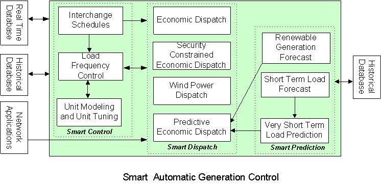
[30] | Chen D, Kumar S, York M, et al. (2012) Smart Automatic Generation Control. IEEE PES General Meeting, 1-6. |
[31] | Chen D, York M (2008) Neural network based approaches to very short term load prediction. IEEE PES General Meeting, 1-8. |
[32] | Chen D, York M (2011) Predictive economic dispatch with time. IEEE PES General Meeting, 1-8. |
[33] | Chen D (1998) Nonlinear neural control with power systems applications. PhD Dissertation, Oregon State University, Corvallis, USA. |
[34] | Vedam R (1994) Nonlinear control applied to power systems. PhD Dissertation, Oregon State University, Corvallis, USA. |
¯CPS1≥100% | ¯CPS1≥120% | ¯CPS1≥135% | |
¯CPS2≥90% | Neural controller 1 NN1 | Neural controller 4 NN4 | Neural controller 7 NN7 |
¯CPS2≥92% | Neural controller 2 NN2 | Neural controller 5 NN5 | Neural controller 8 NN8 |
¯CPS2≥95% | Neural controller 3 NN3 | Neural controller 6 NN6 | Neural controller 9 NN9 |
¯CPS1≥100% | ¯CPS1≥120% | ¯CPS1≥135% | |
BAALv≥15 | Neural controller 1 NN1 | Neural controller 4 NN4 | Neural controller 7 NN7 |
BAALv≥20 | Neural controller 2 NN2 | Neural controller 5 NN5 | Neural controller 8 NN8 |
¯BAALv≥25 | Neural controller 3 NN3 | Neural controller 6 NN6 | Neural controller 9 NN9 |
RMS Error (%) for Training Performance | RMS Error (%) for Prediction Performance | |
Area Regulation for NN1 | 1.823% | 1.835% |
Area Regulation for NN3 | 1.967% | 1.974% |
Area Regulation for NN4 | 1.978% | 1.995% |
Area Regulation for NN6 | 2.107% | 2.254% |
¯CPS1≥100% | ¯CPS1≥120% | ¯CPS1≥135% | |
¯CPS2≥90% | Neural controller 1 NN1 | Neural controller 4 NN4 | Neural controller 7 NN7 |
¯CPS2≥92% | Neural controller 2 NN2 | Neural controller 5 NN5 | Neural controller 8 NN8 |
¯CPS2≥95% | Neural controller 3 NN3 | Neural controller 6 NN6 | Neural controller 9 NN9 |
¯CPS1≥100% | ¯CPS1≥120% | ¯CPS1≥135% | |
BAALv≥15 | Neural controller 1 NN1 | Neural controller 4 NN4 | Neural controller 7 NN7 |
BAALv≥20 | Neural controller 2 NN2 | Neural controller 5 NN5 | Neural controller 8 NN8 |
¯BAALv≥25 | Neural controller 3 NN3 | Neural controller 6 NN6 | Neural controller 9 NN9 |
RMS Error (%) for Training Performance | RMS Error (%) for Prediction Performance | |
Area Regulation for NN1 | 1.823% | 1.835% |
Area Regulation for NN3 | 1.967% | 1.974% |
Area Regulation for NN4 | 1.978% | 1.995% |
Area Regulation for NN6 | 2.107% | 2.254% |