How do leading stock markets in America and Europe connect to Asian stock markets? Quantile dynamic connectedness

OlaOluwa S. Yaya; Miao Zhang; Han Xi; Fumitaka Furuoka; OlaOluwa S. Yaya; Miao Zhang; Han Xi; Fumitaka Furuoka

doi:10.3934/QFE.2024019

Quantitative Finance and Economics

2024, Volume 8, Issue 3: 502-531. doi: 10.3934/QFE.2024019

Previous Article Next Article

Research article

How do leading stock markets in America and Europe connect to Asian stock markets? Quantile dynamic connectedness

1.
Economic and Finance Statistics Unit, University of Ibadan, Ibadan, Nigeria
2.
School of International Relations, Xiamen University, Xiamen, China
3.
Asia-Europe Institute, University of Malaya, Kuala Lumpur, Malaysia

Received: 06 February 2024 Revised: 24 July 2024 Accepted: 06 August 2024 Published: 08 August 2024
JEL Codes: G12, G15, C22

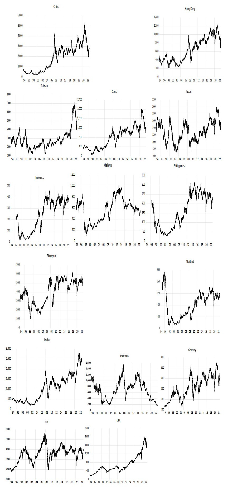
We used the quantile vector autoregressive (QVAR) dynamic connectedness framework to examine whether leading stock markets in America and Europe would have any impact on major stock markets in Asia.¹ More precisely, we analyzed systematically the stock market connectedness in 15 countries, namely Germany, the UK, the USA, and 12 Asian countries, which include five major ASEAN countries, namely Indonesia, Malaysia, Philippines, Singapore, and Thailand from 1996 to 2023. The findings indicated that Hong Kong and Singaporean stocks were major transmitters of financial shocks at the extreme low price market condition, while Germany and UK were minor transmitters. By contrast, the USA could be considered the major transmitter of financial shock during the extreme high market price returns condition. In the normal market condition, these three countries in Europe and America are important transmitters of financial shock. More interestingly, the empirical findings indicated the centrality of Singapore in the stock market connectedness in Asia.
¹ The authors are grateful to Professor David Gabauer who makes available the R codes for all calculations in this paper.
- stock market connectedness,
- Asia,
- Europe,
- America,
- Quantile method,
- extreme high market price returns
Citation: OlaOluwa S. Yaya, Miao Zhang, Han Xi, Fumitaka Furuoka. How do leading stock markets in America and Europe connect to Asian stock markets? Quantile dynamic connectedness[J]. Quantitative Finance and Economics, 2024, 8(3): 502-531. doi: 10.3934/QFE.2024019

Related Papers:

Abstract

We used the quantile vector autoregressive (QVAR) dynamic connectedness framework to examine whether leading stock markets in America and Europe would have any impact on major stock markets in Asia.¹ More precisely, we analyzed systematically the stock market connectedness in 15 countries, namely Germany, the UK, the USA, and 12 Asian countries, which include five major ASEAN countries, namely Indonesia, Malaysia, Philippines, Singapore, and Thailand from 1996 to 2023. The findings indicated that Hong Kong and Singaporean stocks were major transmitters of financial shocks at the extreme low price market condition, while Germany and UK were minor transmitters. By contrast, the USA could be considered the major transmitter of financial shock during the extreme high market price returns condition. In the normal market condition, these three countries in Europe and America are important transmitters of financial shock. More interestingly, the empirical findings indicated the centrality of Singapore in the stock market connectedness in Asia.

¹ The authors are grateful to Professor David Gabauer who makes available the R codes for all calculations in this paper.

References

[1]	Agénor PR, Pereira da Silva LA (2022) Financial spillovers, spillbacks, and the scope for international macroprudential policy coordination. Int Econ Econ Policy 19: 79–127. https://doi.org/10.1007/s10368-021-00522-5 doi: 10.1007/s10368-021-00522-5
[2]	Aggarwal R, Rivoli P (1989) The relationship between the US and four Asian stock markets. ASEAN Econ Bull 6: 110–117.
[3]	Ando T, Greenwood-Nimmo M, Shin Y (2022) Quantile Connectedness: Modeling Tail Behavior in the Topology of Financial Networks. Manag Sci 68: 2401–2431. https://doi.org/10.1287/mnsc.2021.3984 doi: 10.1287/mnsc.2021.3984
[4]	Anscombe FJ, Glynn WJ (1983) Distribution of the kurtosis statistic b2 for normal samples. Biometrika 70: 227–234. https://doi.org/10.1093/biomet/70.1.227 doi: 10.1093/biomet/70.1.227
[5]	Antonakakis N, Chatziantoniou I, Gabauer D (2020) Refined Measures of Dynamic Connectedness based on Time-Varying Parameter Vector Autoregressions. J Risk Financ Manage 13: 84. https://doi.org/10.3390/jrfm13040084 doi: 10.3390/jrfm13040084
[6]	Baig AS, Butt HA, Haroon O, et al. (2021) Deaths, panic, lockdowns and US equity markets: The case of COVID-19 pandemic. Financ Res Lett 38: 101701. https://doi.org/10.1016/j.frl.2020.101701 doi: 10.1016/j.frl.2020.101701
[7]	Balcilar M, Gabauer D, Umar Z (2021) Crude Oil futures contracts and commodity markets: New evidence from a TVP-VAR extended joint connectedness approach. Resour Policy 73: 102219. https://doi.org/10.1016/j.resourpol.2021.102219 doi: 10.1016/j.resourpol.2021.102219
[8]	CEIC (2024) Available from: https://www.ceicdata.com/en (accessed on 7 August 2024)
[9]	Cepoi CO (2020) Asymmetric dependence between stock market returns and news during COVID-19 financial turmoil. Financ Res Lett 36: 101658. https://doi.org/10.1016/j.frl.2020.101658 doi: 10.1016/j.frl.2020.101658
[10]	Chatziantoniou I, Gabauer D (2021) EMU risk-synchronisation and financial fragility through the prism of dynamic connectedness. Q Rev Econ Financ 79: 1–14. https://doi.org/10.1016/j.qref.2020.12.003 doi: 10.1016/j.qref.2020.12.003
[11]	Chatziantoniou I, Gabauer D, Gupta R (2021) Integration and risk transmission in the market for crude oil: a time-varying parameter frequency connectedness approach. Working Paper, University of Portsmouth, No. 202147.
[12]	Chatziantoniou I, Gabauer D, Stenfors A (2021) Interest rate swaps and the transmission mechanism of monetary policy: A quantile connectedness approach. Econ Lett 204: 109891. https://doi.org/10.1016/j.econlet.2021.109891 doi: 10.1016/j.econlet.2021.109891
[13]	Chavleishvili S, Manganelli S (2024) Forecasting and stress testing with quantile vector autoregression. J Appl Economet 39: 66–85. https://doi.org/10.1002/jae.3009 doi: 10.1002/jae.3009
[14]	D'Agostino RB (1970) Transformation to Normality of the Null Distribution of g1. Biometrika 57: 679–681. https://doi.org/10.2307/2334794. doi: 10.2307/2334794
[15]	Dai Z, Zhu J, Zhang X (2022) Time-frequency connectedness and cross-quantile dependence between crude oil, Chinese commodity market, stock market and investor sentiment. Energ Econ 114: 106226. https://doi.org/10.1016/j.eneco.2022.106226. doi: 10.1016/j.eneco.2022.106226
[16]	Diebold FX, Yilmaz K (2009) Measuring financial asset return and volatility spillovers, with application to global equity markets. Econ J 119: 158–171. https://doi.org/10.1111/j.1468-0297.2008.02208.x doi: 10.1111/j.1468-0297.2008.02208.x
[17]	Diebold FX, Yilmaz K (2012) Better to give than to receive: Predictive directional measurement of volatility spillovers. Int J Forecast 28: 57–66. https://doi.org/10.1016/j.ijforecast.2011.02.006 doi: 10.1016/j.ijforecast.2011.02.006
[18]	Diebold FX, Yılmaz K (2014) On the network topology of variance decompositions: Measuring the connectedness of financial firms. J Econometrics 182: 119–134. https://doi.org/10.1016/j.jeconom.2014.04.012 doi: 10.1016/j.jeconom.2014.04.012
[19]	Dornbusch R, Park YC, Claessens S (2000) Contagion: Understanding How It Spreads. World Bank Res Obs 15: 177–197. https://doi.org/10.1093/wbro/15.2.177 doi: 10.1093/wbro/15.2.177
[20]	Elliott G, Rothenberg TJ, Stock JH (1992) Efficient Tests for an Autoregressive Unit Root (Working Paper No. 130) National Bureau of Economic Research. https://doi.org/10.3386/t0130
[21]	Fermanian JD, Scaillet O (2005) Some statistical pitfalls in copula modeling for financial applications. FAME Research paper No.108.
[22]	Fleming JM (1962) Domestic financial policies under fixed and under floating exchange rates. Staff Pap Int Monetary Fund 9: 369–380.
[23]	Fisher TJ, Gallagher CM (2012) New Weighted Portmanteau Statistics for Time Series Goodness of Fit Testing. J Am Stat Assoc 107: 777–787. https://doi.org/10.1080/01621459.2012.688465 doi: 10.1080/01621459.2012.688465
[24]	Furuoka F, Yaya OS, Ling PK, et al. (2023) Transmission of risks between energy and agricultural commodities: Frequency time-varying VAR, asymmetry and portfolio management. Resour Policy 81: 103339. https://doi.org/10.1016/j.resourpol.2023.103339 doi: 10.1016/j.resourpol.2023.103339
[25]	Gautam A, Lepone G (2024) Time Zone Difference and Equity Market Price Efficiency Post Earnings Announcements. http://dx.doi.org/10.2139/ssrn.4815836
[26]	Gabauer D (2021) Dynamic measures of asymmetric & pairwise connectedness within an optimal currency area: Evidence from the ERM I system. J Multinatl Financ M 60: 100680. https://doi.org/10.1016/j.mulfin.2021.100680 doi: 10.1016/j.mulfin.2021.100680
[27]	Grote MH (2007) Mobile marketplaces—consequences of the changing governance of European stock exchanges. Growth Change 38: 260–278. https://doi.org/10.1111/j.1468-2257.2007.00366.x doi: 10.1111/j.1468-2257.2007.00366.x
[28]	Gong C, Tang P, Wang Y (2019) Measuring the network connectedness of global stock markets. Phys A 535: 122351. https://doi.org/10.1016/j.physa.2019.122351 doi: 10.1016/j.physa.2019.122351
[29]	Huang Y, Su W, Li X (2010) Comparison of BEKK GARCH and DCC GARCH models: An empirical study, In: Advanced Data Mining and Applications, Springer Berlin Heidelberg, 99–110. https://doi.org/10.1007/978-3-642-17313-4_10
[30]	Ito T, Krueger AO (2009) Regional and Global Capital Flows: Macroeconomic Causes and Consequences, University of Chicago Press.
[31]	Iwanicz-Drozdowska M, Rogowicz K, Kurowski Ł, et al. (2021) Two decades of contagion effect on stock markets: Which events are more contagious? J Financ Stabil 55: 100907. https://doi.org/10.1016/j.jfs.2021.100907 doi: 10.1016/j.jfs.2021.100907
[32]	Kao EH, Ho TW, Fung HG (2015) Price linkage between the US and Japanese futures across different time zones: An analysis of the minute-by-minute data. J Int Financ Mark I 34: 321–336. https://doi.org/10.1016/j.intfin.2014.12.002 doi: 10.1016/j.intfin.2014.12.002
[33]	Koop G, Pesaran MH, Potter SM (1996) Impulse response analysis in nonlinear multivariate models. J Econometrics 74: 119–147. https://doi.org/10.1016/0304-4076(95)01753-4 doi: 10.1016/0304-4076(95)01753-4
[34]	Korkmaz A (2014) Can the Interdependence Effect and the Contagion Phenomena be Related with One Another? J Empirl Stud 1: 38–47.
[35]	Lin WL, Engle RF, Ito T (1994) Do bulls and bears move across borders? International transmission of stock returns and volatility. Rev Financ Stud 7: 507–538. https://doi.org/10.1093/rfs/7.3.507 doi: 10.1093/rfs/7.3.507
[36]	Mai JF, Scherer M (2013) What makes dependence modeling challenging? Pitfalls and ways to circumvent them. Statist Risk Model 30: 287–306. https://doi.org/10.1524/strm.2013.2001 doi: 10.1524/strm.2013.2001
[37]	Marfatia HA (2017) A Fresh Look at Integration of Risks in the International Stock Markets: A Wavelet Approach. Rev Financ Econ 34: 33–49. https://doi.org/10.1016/j.rfe.2017.07.003 doi: 10.1016/j.rfe.2017.07.003
[38]	Mensi W, Boubaker FZ, Al-Yahyaee KH, et al. (2018) Dynamic volatility spillovers and connectedness between global, regional, and GIPSI stock markets. Financ Res Lett 25: 230–238. https://doi.org/10.1016/j.frl.2017.10.032 doi: 10.1016/j.frl.2017.10.032
[39]	Mensi W, Ziadat SA, Vo XV, et al. (2024) Extreme quantile connectedness and spillovers between oil and Vietnamese stock markets: a sectoral analysis. Int J Emerg Mark 19: 1586–1625. https://doi.org/10.1108/IJOEM-03-2022-0513 doi: 10.1108/IJOEM-03-2022-0513
[40]	Mishkin FS (1999) Lessons from the Asian crisis. J Int Money Financ 18: 709–723. https://doi.org/10.1016/S0261-5606(99)00020-0 doi: 10.1016/S0261-5606(99)00020-0
[41]	Noble GW, Ravenhill J (2000) Causes and Consequences of the Asian Financial Crisis, In: G. W. Noble & J. Ravenhill (Eds.), The Asian Financial Crisis and the Architecture of Global Finance Cambridge University Press, 1st ed., 1–35. https://doi.org/10.1017/CBO9781139171328.002
[42]	Pesaran HH, Shin Y (1998) Generalized impulse response analysis in linear multivariate models. Econ Lett 58: 17–29. https://doi.org/10.1016/S0165-1765(97)00214-0 doi: 10.1016/S0165-1765(97)00214-0
[43]	S&P Global (2023) S&Q Capital IQ. https://www.spglobal.com/marketintelligence/. [accessed on 25 February 2023].
[44]	Samarakoon LP (2011) Stock market interdependence, contagion, and the US financial crisis: The case of emerging and frontier markets. J Int Financ Mark I 21: 724–742. https://doi.org/10.1016/j.intfin.2011.05.001 doi: 10.1016/j.intfin.2011.05.001
[45]	Serrano P, Vaello-Sebastià A, Vich-Llompart MM (2023) The international linkages of market risk perception. J Multinatl Financ M 72: 100826. https://doi.org/10.1016/j.mulfin.2023.100826 doi: 10.1016/j.mulfin.2023.100826
[46]	Schüler YS (2014) Asymmetric effects of uncertainty over the business cycle: A quantile structural vector autoregressive approach. Universi ty of Konstanz, Department of Economics, Working Paper No. 2014-0.
[47]	Tiwari AK, Abakah EJA, Yaya OS, et al. (2022) Tail risk dependence, co-movement and predictability between green bond and green stocks. Appl Econ 55: 201–222. https://doi.org/10.1080/00036846.2022.2085869 doi: 10.1080/00036846.2022.2085869
[48]	Tuominen DR (2020) Investigation on how Brexit has impacted IPO listings with Deutsche Börse and the London Stock Exchange. Degree Thesis, Arcada University of Applied Sciences (Finland). Available from: https://www.theseus.fi/handle/10024/353824 (accessed on 6 April 2024)
[49]	Ullah S (2015) The Impact of Internal Corporate Governance Mechanisms on the Performance of Firms: Evidence from the UK and Germany. Open University (United Kingdom). Available from: https://www.proquest.com/docview/2171038131?pq-origsite = gscholar & fromopenview = true & sourcetype = Dissertations%20 & %20Theses(accessed on 7 February 2024)
[50]	Wang P, Wang P (2010) Price and volatility spillovers between the Greater China Markets and the developed markets of US and Japan. Global Financ J 21: 304–317. https://doi.org/10.1016/j.gfj.2010.09.007
[51]	Yang Z, Zhou Y (2017) Quantitative easing and volatility spillovers across countries and asset classes. Manage Sci 63: 333–354. https://doi.org/10.1287/mnsc.2015.2305 doi: 10.1287/mnsc.2015.2305
[52]	Yousaf I, Mensi W, Vo XV, et al. (2023) Spillovers and connectedness between Chinese and ASEAN stock markets during bearish and bullish market statuses. Int J Emerg Mark. https://doi.org/10.1108/IJOEM-07-2022-1194 doi: 10.1108/IJOEM-07-2022-1194
[53]	Yuce A, Simga-Mugan C (2000) Linkages among Eastern European stock markets and the major stock exchanges. Russian East Eur Financ Trade 36: 54–69.
[54]	Zhang Q, Wei R (2024) Carbon reduction attention and financial market stress: A network spillover analysis based on quantile VAR modeling. J Environ Manage 356: 120640. https://doi.org/10.1016/j.jenvman.2024.120640 doi: 10.1016/j.jenvman.2024.120640

QFE-08-03-019-s001.pdf

Reader Comments

Your name:*

Email:*
© 2024 the Author(s), licensee AIMS Press. This is an open access article distributed under the terms of the Creative Commons Attribution License (http://creativecommons.org/licenses/by/4.0)