Encephalomalacia/gliosis, deep venous thrombosis, and cancer in Arg393His antithrombin Hanoi and the potential impact of the β-amyloid precursor protein (APP) on thrombosis and cancer

Khue Vu Nguyen; Khue Vu Nguyen

doi:10.3934/Neuroscience.2022010

AIMS Neuroscience

2022, Volume 9, Issue 2: 175-215. doi: 10.3934/Neuroscience.2022010

Previous Article Next Article

Review

Encephalomalacia/gliosis, deep venous thrombosis, and cancer in Arg393His antithrombin Hanoi and the potential impact of the β-amyloid precursor protein (APP) on thrombosis and cancer

Khue Vu Nguyen ^{1,2
,
,}

Former Institution Attended:
1.
Department of Medicine, Biochemical Genetics and Metabolism, The Mitochondrial and Metabolic Disease Center, School of Medicine, University of California, San Diego, Building CTF, Room C-103, 214 Dickinson Street, San Diego, CA 92103-8467, USA
2.
Department of Pediatrics, University of California, San Diego, School of Medicine, San Diego, La Jolla, CA 92093-0830, USA

Received: 25 October 2021 Revised: 15 April 2022 Accepted: 18 April 2022 Published: 21 April 2022

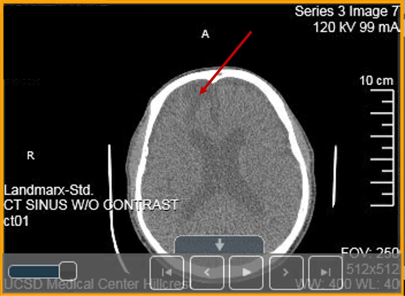
A heterozygous Arg393His point mutation at the reactive site of antithrombin (AT) gene causing thrombosis in a Vietnamese patient is reported and named as Arg393His in AT-Hanoi. The present variant is characterized by a severe reduction of functionally active AT plasma concentration to 42% of normal resulting in multiple severe thrombotic events such as cerebral venous thrombosis (CVT) (encephalomalacia/gliosis), recurrent deep venous thrombosis (DVT) and the development of kidney cancer. Today the complexity of thrombophilia has grown with appreciation that multiple inherited and acquired risk factors may interact to result in a clinically thrombotic phenotype. This article focuses on the following issues: (1) pathophysiology and clinical conditions of Arg393His in AT-Hanoi; (2) “two way association” between cancer and thrombosis in which venous thromboembolism (VTE) can be both a presenting sign and a complication of cancer; (3) efficacy of anticoagulants used for the prevention of cancer-related thrombosis; (4) conditions of acquired risk factors such as cancer or genetic disorders via epigenetic modifications in gene-gene (epistasis) and/or gene-environment interactions such as in Lesch-Nyhan disease (LND), in which the β-amyloid precursor protein (APP) that may interact to predispose a patient to thrombosis and cancer. It is also necessary to study the hypoxanthine-guanine phosphoribosyltransferase (HGprt) enzyme, AT, and APP using expression vectors for exploring their impact on LND, thrombosis as well as other human diseases, especially the ones related to APP such as Alzheimer's disease (AD) and cancer. For such a purpose, the construction of expression vectors for HGprt and APP, with or without the glycosyl-phosphatidylinositol (GPI) anchor, was performed as described in Ref. #148 (Nguyen, K. V., Naviaux, R. K., Nyhan, W. L. Lesch-Nyhan disease: I. Construction of expression vectors for hypoxanthine-guanine phosphoribosyltransferase (HGprt) enzyme and amyloid precursor protein (APP). Nucleosides Nucleotides Nucleic Acids 2020, 39: 905–922). In the same manner, the construction of expression vectors for AT and APP can be performed as shown in Figure 6. These expressions vectors, with or without GPI anchor, could be used as tools for (a) studying the effects of Arg393His mutation in AT; (b) studying the emerging role of Arg393His mutation in AT and cancer; (c) studying intermolecular interactions between APP and AT.

Furthermore, the construction of expression vectors as described in Ref. #148, especially the one with GPI, can be used as a model for the construction of expression vectors for any protein targeting to the cell plasma membrane for studying intermolecular interactions and could be therefore useful in the vaccines as well as antiviral drugs development (studying intermolecular interactions between the spike glycoprotein of the severe acute respiratory syndrome coronavirus 2, SARS-CoV-2, as well as its variants and the angiotensin-converting enzyme 2, ACE2, in coronavirus disease 2019 (COVID-19) [155],[156], for example).
Citation: Khue Vu Nguyen. Encephalomalacia/gliosis, deep venous thrombosis, and cancer in Arg393His antithrombin Hanoi and the potential impact of the β-amyloid precursor protein (APP) on thrombosis and cancer[J]. AIMS Neuroscience, 2022, 9(2): 175-215. doi: 10.3934/Neuroscience.2022010

Related Papers:

Abstract

A heterozygous Arg393His point mutation at the reactive site of antithrombin (AT) gene causing thrombosis in a Vietnamese patient is reported and named as Arg393His in AT-Hanoi. The present variant is characterized by a severe reduction of functionally active AT plasma concentration to 42% of normal resulting in multiple severe thrombotic events such as cerebral venous thrombosis (CVT) (encephalomalacia/gliosis), recurrent deep venous thrombosis (DVT) and the development of kidney cancer. Today the complexity of thrombophilia has grown with appreciation that multiple inherited and acquired risk factors may interact to result in a clinically thrombotic phenotype. This article focuses on the following issues: (1) pathophysiology and clinical conditions of Arg393His in AT-Hanoi; (2) “two way association” between cancer and thrombosis in which venous thromboembolism (VTE) can be both a presenting sign and a complication of cancer; (3) efficacy of anticoagulants used for the prevention of cancer-related thrombosis; (4) conditions of acquired risk factors such as cancer or genetic disorders via epigenetic modifications in gene-gene (epistasis) and/or gene-environment interactions such as in Lesch-Nyhan disease (LND), in which the β-amyloid precursor protein (APP) that may interact to predispose a patient to thrombosis and cancer. It is also necessary to study the hypoxanthine-guanine phosphoribosyltransferase (HGprt) enzyme, AT, and APP using expression vectors for exploring their impact on LND, thrombosis as well as other human diseases, especially the ones related to APP such as Alzheimer's disease (AD) and cancer. For such a purpose, the construction of expression vectors for HGprt and APP, with or without the glycosyl-phosphatidylinositol (GPI) anchor, was performed as described in Ref. #148 (Nguyen, K. V., Naviaux, R. K., Nyhan, W. L. Lesch-Nyhan disease: I. Construction of expression vectors for hypoxanthine-guanine phosphoribosyltransferase (HGprt) enzyme and amyloid precursor protein (APP). Nucleosides Nucleotides Nucleic Acids 2020, 39: 905–922). In the same manner, the construction of expression vectors for AT and APP can be performed as shown in Figure 6. These expressions vectors, with or without GPI anchor, could be used as tools for (a) studying the effects of Arg393His mutation in AT; (b) studying the emerging role of Arg393His mutation in AT and cancer; (c) studying intermolecular interactions between APP and AT.

Furthermore, the construction of expression vectors as described in Ref. #148, especially the one with GPI, can be used as a model for the construction of expression vectors for any protein targeting to the cell plasma membrane for studying intermolecular interactions and could be therefore useful in the vaccines as well as antiviral drugs development (studying intermolecular interactions between the spike glycoprotein of the severe acute respiratory syndrome coronavirus 2, SARS-CoV-2, as well as its variants and the angiotensin-converting enzyme 2, ACE2, in coronavirus disease 2019 (COVID-19) [155],[156], for example).

Abbreviations

Aβ

β-amyloid peptide

ACE2

angiotensin-converting enzyme 2

ACT

activated clotting time

Alzheimer's disease

APC

activated protein C

aPL

antiphospholipid

APLP1

β-amyloid precursor-like protein 1

APLP2

β-amyloid precursor-like protein 2

APP

β-amyloid precursor protein

APP-mRNA

β-amyloid precursor protein messenger RNA

APPsα

soluble APP fragment released from APP following the cleavage by α-secretase

aPTT or APTT

activated partial thromboplastin time

alternative splicing

ASCO

American society of clinical oncology

anthithrombin

AT I

antithrombin I

AT II

antithrombin II

AT III

antithrombin III

AT IV

antithrombin IV

ATP

adenosine-5′-triphosphate

CAPS

catastrophic antiphospholipid syndrome

cdk2

cyclin-dependent kinase 2

COVID-19

coronavirus disease 2019

CNS

central nervous system

computed tomography

CTA

computed tomography angiography

CUS

compression ultrasound

CVT

cerebral venous thrombosis

DVT

deep venous thrombosis

EGFR-R776H

epidermal growth factor receptor-Arg776His

FFP

fresh frozen plasma

GPI

glycosyl-phosphatidylinositol

GTP

guanosine-5′-triphosphate

HBS

heparin binding site

HDM2

human homologue of the murine double minute 2 protein

HGprt

hypoxanthine-guanine phosphoribosyltransferase

HIT

heparin-induced thrombocytopenia

HIV

human immunodeficiency virus

HND

HGprt-related neurological dysfunction

HPRT1

hypoxanthine phosphoribosyltransferase 1

HPRT1-mRNA

hypoxanthine phosphoryltransferase 1 messenger RNA

HRH

HGprt-related hyperuricemia

INDELS

deletion followed by an insertion

INR

international normalized ratio

KPI

Kunitz protease inhibitor

LMWH

low-molecular-weight heparin

LND

Lesch-Nyhan disease

LNV

Lesch-Nyhan variant

MIM

Mendelian inheritance in man

mRNA

messenger RNA

NET

neutrophil extracellular trap

NOAC

non-vitamin K antagonist oral anticoagulant

NSAID

nonsteroidal anti-inflammatory drug

P21/WAF1

also known as cyclin-dependent kinase inhibitor 1 or CDK-interacting; protein 1, is a cyclin-dependent kinase inhibitor (CKI) that is capable; of inhibiting all cyclin/CDK complexes, and thus function as a regulator; of cell cycle progression at G1 and S phase

PCR

polymerase chain reaction

pharmacodynamics

pulmonary embolism

pHi

pH intracellular

pharmacokinetics

PN-2

protease nexin-2

prothrombin time

PTT

partial thromboplastin time

reactive site

SARS-CoV-2

severe acute respiratory syndrome coronavirus 2

siRNA

small interfering RNA

TAD

trans-activation domain

tissue factor

TFPI

tissue factor pathway inhibitor

TK1

thymidine kinase 1

TP53

tumor suppressor protein 53

UFH

unfractionated heparin

VKA

vitamin K antagonist

VTE

venous thromboembolism

WARF

Wisconsin alumni research foundation

WNV

West Nile virus

Conflict of interest

The authors declare no conflict of interest.

References

[1]	Seegers WH, Johnson JF, Fell C (1954) An antthrombin reaction to prothrombin activation. Am J Physiol 176: 97-103. https://doi.org/10.1152/ajplegacy.1953.176.1.97
[2]	Egeberg O (1965) Inherited antithrombin deficiency causing thrombophilia. Thromb Diath Haemorrh 13: 516-530. https://doi.org/10.1055/s-0038-1656297
[3]	Griffin JH, Evatt B, Zimmerman TS, et al. (1981) Deficiency of protein C in congenital thrombotic disease. J Clin Invest 68: 1370-1373. https://doi.org/10.1172/JCI110385
[4]	Comp PC, Esmon C (1984) Recurrent venous thromboembolism in patients with a partial deficiency of protein S. N Engl J Med 311: 1525-1528. https://doi.org/10.1056/NEJM198412133112401
[5]	Schwarz HP, Fischer M, Hopmeier P, et al. (1984) Plasma protein S deficiency in familial thrombotic disease. Blood 64: 1297-1300. https://doi.org/10.1182/blood.V64.6.1297.1297
[6]	Conard J, Brosstad F, Lie Larsen M, et al. (1983) Molar antithrombin concentration in normal human plasma. Haemostasis 13: 363-368. https://doi.org/10.1159/000214823
[7]	Collen D, Schetz J, de Cock F, et al. (1977) Holmer, E., Verstraete, M. Metabolism of antithrombin III (heparin cofactor) in man: effects of venous thrombosis of heparin administration. Eur J Clin Invest 7: 27-35. https://doi.org/10.1111/j.1365-2362.1977.tb01566.x
[8]	Maclean PS, Tait RC (2007) Hereditary and acquired antithrombin deficiency: epidemiology, pathogenesis and treatment options. Drugs 67: 1429-1440. https://doi.org/10.2165/00003495-200767100-00005
[9]	Wells PS, Blajchman MA, Henderson P, et al. (1994) Prevalence of antithrombin deficiency in healthy blood donors: a cross-sectional study. Am J Hematol 45: 321-324. https://doi.org/10.1002/ajh.2830450409
[10]	Tait RC, Walker ID, Perry DJ, et al. (1994) Prevalence of antithrombin deficiency in the healthy population. Br J Haematol 87: 106-112. https://doi.org/10.1111/j.1365-2141.1994.tb04878.x
[11]	Picard V, Nowark-Gottl U, Biron-Andreani C, et al. (2006) Molecular bases of antithrombin deficiency: twenty-two novel mutations in the antithrombin gene. Hum Mutat 27: 600. https://doi.org/10.1002/humu.9425
[12]	Khor B, Van Cott EM (2010) Laboratory tests for antithrombin deficiency. Am J Hematol 85: 947-950. https://doi.org/10.1002/ajh.21893
[13]	Patnaik MM, Moll S (2008) Inherited antithrombin deficiency: a review. Haemophilia 14: 1229-1239. https://doi.org/10.1111/j.1365-2516.2008.01830.x
[14]	Dahlback B (2008) Advances in understanding pathogenic mechanisms of thrombophilic disorders. Blood 112: 19-27. https://doi.org/10.1182/blood-2008-01-077909
[15]	Rodgers GM (2009) Role of antithrombin concentrate in treatment of hereditary antithrombin deficiency. An update. Thromb Haemost 101: 806-812. https://doi.org/10.1160/TH08-10-0672
[16]	Nguyen KV (2012) Antithrombin Hanoi: Arg393 to His missense point mutation in antithrombin gene and cancer. WebmedCentral: International Journal of Medicine and Molecular Medicine 3: WMC003720.
[17]	Bock SC (2001) Anthithrombin III and heparin cofactor II. Hemostasis and Thrombosis: Basic Principles and Clinical Practice. Philadelphia, Pa: Lippincott Williams & Wilkins: pp. 321-333.
[18]	Walker CPR, Royston D (2002) Thrombin generation and its inhibition: a review of the scientific basis and mechanism of action of anticoagulant therapies. Br J Anaesth 88: 848-863. https://doi.org/10.1093/bja/88.6.848
[19]	Morawitz P (1905) Die Chemie der Blutgerinnung. Ergeb Physiol 4: 307-319. https://doi.org/10.1007/BF02321003
[20]	Quick AJ (1938) The normal antithrombin of the blood and its relation to heparin. Am J Physiol 123: 712-719. https://doi.org/10.1152/ajplegacy.1938.123.3.712
[21]	Fell C, Ivanovic N, Johnson SA, et al. (1954) Differenciation of plasma antithrombin activities. Proc Soc Exp Biol Med 85: 199-202. https://doi.org/10.3181/00379727-85-20829
[22]	Sakuragawa N (1997) Regulation of thrombosis and hemostasis by antithrombin. Semin Thromb Hemost 23: 557-562. https://doi.org/10.1055/s-2007-996136
[23]	Mammen EF (1998) Antithrombin: its physiological importance and role in DIC. Semin Thromb Hemost 24: 19-25. https://doi.org/10.1055/s-2007-995819
[24]	Bock SC, Harris JF, Balazs I, et al. (1985) Assignment of the human antithrombin III structural gene to chromosome 1q23-25. Cytogenet Cell Genet 39: 67-69. https://doi.org/10.1159/000132105
[25]	Olds RJ, Lane DA, Chowdhury V, et al. (1993) Complete nucleotide sequence of the antithrombin gene: evidence for homologous recombination causing thrombophilia. Biochemistry 32: 4216-4224. https://doi.org/10.1021/bi00067a008
[26]	Van Boven HH, Lane DA (1997) Antithrombin and its inherited deficiency states. Semin Hematol 34: 188-204.
[27]	Bock SC, Marriman JA, Radziejewska E (1998) Antithrombin III Utah: proline- 407 to leucine mutation in a highly conserved region near the inhibitor reactive site. Biochemistry 27: 6171-6178. https://doi.org/10.1021/bi00416a052
[28]	Petersen TE, Dulek-Wojciechowski G, Sottrup-Jensen L, et al. (1979) Primary structure of antithrombin III (heparin cofactor): partial homology between alpha 1 antitrypsin and antithrombin III. The physiology inhibitors of blood coagulation and fibrinolysis. Amsterdam, The Netherlands: Elsevier Science: pp. 43-54.
[29]	Bock SC, Wion KL, Vehar GA, et al. (1982) Cloning and expression of the cDNA for human antithrombin III. Nucleic Acids Res 10: 8113-8125. https://doi.org/10.1093/nar/10.24.8113
[30]	Prochownik EV, Orkin SH (1984) In vivo transcription of a human antithrombin III “minigene”. J Biol Chem 259: 15386-15392. https://doi.org/10.1016/S0021-9258(17)42561-0
[31]	Patston PA, Gettins P, Beechem J, et al. (1991) Mechanism of serpin action: evidence thet C1 inhibitor functions as a suicide substrate. Biochemistry 30: 8876-8882. https://doi.org/10.1021/bi00100a022
[32]	Bjork J, Jackson CM, Jornvall H, et al. (1982) The active site of antithrombin. Release of the same proteolytically cleaved form of the inhibitor from complexes with factor IXa, factor Xa, and thrombin. J Biol Chem 257: 2406-2411. https://doi.org/10.1016/S0021-9258(18)34938-X
[33]	Marchant KK, Ducan A (2002) Antithrombin deficiency. Issue in laboratory diagnosis. Arch Pathol Lab Med 126: 1326-1336. https://doi.org/10.5858/2002-126-1326-AD
[34]	Perry DJ (1994) Antithrombin and its inherited deficiencies. Blood Rev 8: 37-55. https://doi.org/10.1016/0268-960X(94)90006-X
[35]	Lane DA, Olds RJ, Thein SL (1994) Antithrombin and its deficiency. Hemostasis and thrombosis. Edinburgh: Churchils Livingstone: pp. 655-670.
[36]	Hirsh J, Piovella F, Pini M (1989) Congenital antithrombin III deficiency: incidence and clinical features. Am J Med 87: 34S-38S. https://doi.org/10.1016/0002-9343(89)80529-7
[37]	Koide T, Odani S, Takahashi K, et al. (1984) Antithrombin III Toyama: replacement of arginine-47 by cysteine in hereditary abnormal antithrombin III that lacks heparin-binding ability. Proc Natl Acad Sci USA 81: 289-293. https://doi.org/10.1073/pnas.81.2.289
[38]	Chang JY, Tran TH (1986) Antithrombin III Basel. Identification of a pro-leu substitution in a hereditary abnormal antithrombin with impaired heparin cofactor activity. J Biol Chem 261: 1174-1176. https://doi.org/10.1016/S0021-9258(17)36071-4
[39]	Owen MC, Borg JY, Soria C, et al. (1987) Heparin binding defect in a new antithrombin III variant: Rouen, 47 Arg to His. Blood 69: 1275-1279. https://doi.org/10.1182/blood.V69.5.1275.1275
[40]	Stephens AW, Thalley BS, Hirs CHW (1987) Antithrombin-III Denver, a reactive site variant. J Biol Chem 262: 1044-1048. https://doi.org/10.1016/S0021-9258(19)75747-0
[41]	Lane DA, Flynn A, Ireland H, et al. (1987) Antithrombin III Nortwick Park: demonstration of an inactive high MW complex with increased affinity for heparin. Br J Haematol 65: 451-456. https://doi.org/10.1111/j.1365-2141.1987.tb04149.x
[42]	Erdjument H, Lane DA, Ireland H, et al. (1987) Formation of a covalent disulfide- linked antithrombin-albumin complex by an antithrombin variant, antithrombin “Northwick Park”. J Biol Chem 262: 13381-13384. https://doi.org/10.1016/S0021-9258(19)76436-9
[43]	Lane DA, Lowe GDO, Flynn A, et al. (1987) Antithrombin III Glasgow: a variant with increased heparin affinity and reduced ability to inactivate thrombin, associated with familial thrombosis. Br J Haematol 66: 523-527. https://doi.org/10.1111/j.1365-2141.1987.tb01338.x
[44]	Owen MC, Beresford CH, Carrell RW (1988) Antithrombin Glasgow, 393 Arg to His: a P1 reactive site variant with increased heparin affinity but no thrombin inhibitory activity. FEBS Lett 231: 317-320. https://doi.org/10.1016/0014-5793(88)80841-X
[45]	Lane DA, Erdjument AF, Flynn A, et al. (1989) Antithrombin Sheffield: amino acid substitution at the reactive site (Arg393 to His) causing thrombosis. Br J Haematol 71: 91-96. https://doi.org/10.1111/j.1365-2141.1989.tb06280.x
[46]	Kenji O, Hiroki A, Masako W, et al. (1995) Antithrombin III Kumamoto: a single mutation at Arg393-His increases the affinity of Antithrombin III for heparin. Am J Hematol 48: 12-18. https://doi.org/10.1002/ajh.2830480104
[47]	Ulivi L, Squitieri M, Cohen H, et al. (2020) Cerebral venous thrombosis: a practical guide. Pract Neurol 20: 356-367. https://doi.org/10.1136/practneurol-2019-002415
[48]	Betts MJ, Russell RB (2003) Amino acid properties and consequences of substitutions. Bioinformatics for geneticists.John Wiley & Sons, Ltd: pp. 289-316. https://doi.org/10.1002/0470867302.ch14
[49]	Kyrle PA, Minar E, Hirschl M, et al. (2000) High plasma levels of Factor VIII and the risk of recurrent venous thromboembolism. N Engl J Med 343: 457-462. https://doi.org/10.1056/NEJM200008173430702
[50]	Kamphuisen PW, Eikenboom JCJ, Bertina RM (2001) Elevated factor VIII levels and the risk of thrombosis. Arterioscler Thromb Vasc Biol 21: 731-738. https://doi.org/10.1161/01.ATV.21.5.731
[51]	Garcia JH, Williams JP, Tanaka J (1975) Spontaneous thrombosis of deep cerebral veins: a complication of arteriovenous malformation. Stroke 6: 164-171. https://doi.org/10.1161/01.STR.6.2.164
[52]	Shah Sid “Stroke pathophysiology.” Foundation for education and research in neurological emergencies. [FERNE]: 1–14. web (2013). Available from: http://tigger.uic.edu/com/ferne/pdf2/saem_0501/shah_stroke_0501.pdf
[53]	Ord-Mackenzi SA (1898) Transient and recurring paresis in acute cerebral softening. Br Med J 1: 140. https://doi.org/10.1136/bmj.1.1933.140
[54]	Fourrier F, Lestavel P, Chopin C, et al. (1990) Meningococcemia and purpura fulminants in adults: acute deficiencies of proteins C and S and early treatment with antithrombin III concentrates. Intensive Care Med 16: 121-124. https://doi.org/10.1007/BF02575306
[55]	Bozzola E, Bozzola M, Colafati GS, et al. (2014) Multiple cerebral sinus thromboses complicating meningococcal meningitis: a pediatric case report. BMC Pediatrics 14: 147. https://doi.org/10.1186/1471-2431-14-147
[56]	Fawcett JW, Asher RA (1999) The glial scar and central nervous system repair. Brain Res Bull 49: 377-391. https://doi.org/10.1016/S0361-9230(99)00072-6
[57]	Heparin antifactor Xa assay (2009). (http://www2.massgeneral.org/pathology/coagbook/CO005000.htm) Archived (https://archive.is/20090808194520/ http://www2.massgeneral.org/pathology/coagbook/CO005000.htm) 2009- 08-08 at Archive.today Page Updated: September 18, 2009
[58]	Refael M, Xing L, Lim W, et al. (2017) Management of venous thromboembolism in patients with hereditary antithrombin deficiency and pregnancy: case report and review of the literature. Case Rep Hematol : Article ID: 9261351. https://doi.org/10.1155/2017/9261351
[59]	Ansell J, Hirsh, Hylek E, et al. (2008) Pharmacology and management of the vitamin K antagonists: American college Chest physicians evidence-based clinical practice guidelines (8^th edition). Chest 133: 160S-198S. https://doi.org/10.1378/chest.08-0670
[60]	Ageno W, Gallus AS, Wittkowsky A, et al. (2012) Oral anticoagulant therapy: antithrombotic therapy and prevention of thrombosis, 9^th ed.: American college Chest physicians evidence-based clinical 141: practice guidelines. Chest 141: e44S-e88S. https://doi.org/10.1378/chest.11-2292
[61]	. Coumadin (https//www.drugs.com/monograph/coumadin.htlm). The American society of health-system pharmacists. Archived (https//web.archive.org/web/20110203081242/ http://www.drugs.com/monograph/coumadin.html) from the original on 3 February 2011. Retrieved 3 April 2011.
[62]	. Warfarin sodium (https://www.drugs.com/monograph/warfarin-sodium.html). The American society of health-system pharmacists. Archived (https://web.archive.org/web/20180612143838/ https://www.drugs.com/monograph/warfarin-sodium.html) from the original on 12 June 2018. Retrieved 8 January 2017.
[63]	Weathermor R, Crabb DW (1999) Alcohol and medication interactions. Alcohol Res Health 23: 40-54.
[64]	Clinically significant drug interactions - American family physician (2016). (http://www.aafp.org/afp/2000/0315/p1745.html#sec-1) Archived (https://web.archive.org/web/20160507065339/http://www.aafp.org/afp/2000/0315/p1745.html) 7 May 2016 at the Wayback Machine
[65]	Wang KL, Yap ES, Goto S, et al. (2018) The diagnosis and treatment of venous thromboembolism in Asian patients. Thromb J 16: 4. https://doi.org/10.1186/s12959-017-0155-z
[66]	Darvall KAL, Sam RC, Silverman SH, et al. (2007) Obesity and thrombosis. Eur J Vasc Surg 33: 223-233. https://doi.org/10.1016/j.ejvs.2006.10.006
[67]	Ridker PM, Miletich JP, Hennekens CH, et al. (1997) Ethnic distribution of factor V Leiden in 4047 men and women. Implications for venous thromboembolism screening. JAMA 277: 1305-1307. https://doi.org/10.1001/jama.1997.03540400055031
[68]	Varga EA, Moll S (2004) Prothrombin 20210 mutation (factor II mutation). Circulation 110: e15-e18. https://doi.org/10.1161/01.CIR.0000135582.53444.87
[69]	Weinberger J, Cipolle M (2016) Mechanism prophylaxix for post-traumatic VTE: stockings and pumps. Curr Trauma Rep 2: 35-41. https://doi.org/10.1007/s40719-016-0039-x
[70]	Liew NC, Chang YH, Choi G, et al. (2012) Asian venous thrombosis forum. Asian venous thromboembolism guidelines: prevention of venous thromboembolism. Int Angiol 31: 501-516.
[71]	ISTH Steering Committee for World Thrombosis Day.Thrombosis: a major contributor to global disease burden. Thromb Haemost (2014) 112: 843-852. https://doi.org/10.1160/th14-08-0671
[72]	Hotoleanu C (2020) Association between obesity and venous thromboembolism. Med Pharm Rep 93: 162-168. https://doi.org/10.15386/mpr-1372
[73]	Aksu K, Donmez A, Keser G (2012) Inflammation-induced thrombosis: mechanism, disease associations management. Curr Pharma Des 18: 1478-1493. https://doi.org/10.2174/138161212799504731
[74]	Middellorp S, Coppens M, van Happs F (2020) Incidence of venous thromboembolism in hospitalized patients with COVID-19. J Thromb Haemost 18: 1995-2002. https://doi.org/10.1111/jth.14888
[75]	Connors JM, Levy JH (2020) COVID-19 and its implications for thrombosis and anticoagulation. Blood 135: 2033-2040. https://doi.org/10.1182/blood.2020006000
[76]	Vinogradova Y, Coupland C, Hippisley-Cox J (2019) Use of hormone replacement therapy and risk of venous thromboembolism: nested case-control studies using the QResearch and CPRD databases. BMJ 364: k4810. https://doi.org/10.1136/bmj.k4810
[77]	Ye F, Bell LN, Mazza J, et al. (2018) Variation in definitions of immobility in pharmacological thromboprophylaxis clinical trials in medical inpatients: a systemic review. Clin Appl Thromb Hemost 24: 13-21. https://doi.org/10.1177/1076029616677802
[78]	Fernandes CJ, Morinaga LTK, Alves JL, et al. (2019) Cancer-associated thrombosis: the when, how and why. Eur Respir Rev 28: 180119. https://doi.org/10.1183/16000617.0119-2018
[79]	Noble S, Pasi J (2010) Epidemiology and pathophysiology of cancer-associated thrombosis. Br J Cancer 102: S2-S9. https://doi.org/10.1038/sj.bjc.6605599
[80]	Bouillaud JB, Bouillaud S (1823) De l'Obliteration des veines et de son influence sur la formation des hydropisies partielles: consideration sur la hydropisies passive et general. Arch Gen Med 1: 188-204.
[81]	Trousseau A (1865) Phlegmasia alba dolens. Clinique medicale de l'Hotel- Dieu de Paris. Paris: Balliere: pp. 654-712.
[82]	Trousseau A (1877) Ulcere chronique simple de l'estomac. Clinique medicale de l'Hotel-Dieu de Paris. Paris: Bailliere J.-B. et fils: pp. 80-107.
[83]	Trousseau A (1877) Phlegmasia alba dolens. Clinique medicale de l'Hotel-Dieu de Paris. Paris: Bailliere J.-B. et fils: pp. 695-739.
[84]	Illtyd James T, Matheson N (1935) Thromboplebitis in cancer. Practitioner 134: 683-684.
[85]	Gore JM, Appelbaum JS, Greene HL, et al. (1982) Occult cancer in patients with acute pulmonary embolism. Ann Intern Med 96: 556-560. https://doi.org/10.7326/0003-4819-96-5-556
[86]	Prandoni P, Lensing AWA, Buller HR, et al. (1992) Deep-vein thrombosis and the incidence of subsequent symptomatic cancer. N Engl J Med 327: 1128-1133. https://doi.org/10.1056/NEJM199210153271604
[87]	Lee AYY, Levine MN (2003) Venous thrombosis and cancer: risks and outcomes. Circulation 107: I-17-I-21. https://doi.org/10.1161/01.CIR.0000078466.72504.AC
[88]	Dotsenko O, Kakkar AK (2006) Thrombosis and cancer. Ann Oncol 17: x81-x84. https://doi.org/10.1093/annonc/mdl242
[89]	Buller HR, Van Doormaal FF, Van Sluis GL, et al. (2007) Cancer and thrombosis: from molecular mechanisms to clinical presentations. J Thromb Haemost 5: 246-254. https://doi.org/10.1111/j.1538-7836.2007.02497.x
[90]	Sorensen HT, Mellemkjaer L, Olsen JH, et al. (2000) Prognosis of cancers associated with venous thromboembolism. N Engl J Med 343: 1846-1850. https://doi.org/10.1056/NEJM200012213432504
[91]	Tincani A, Taraborelli M, Cattaneo R (2010) Antiphospholipid antibodies and malignancies. Autoimmun Rev 9: 200-202. https://doi.org/10.1016/j.autrev.2009.04.001
[92]	Angchaisuksiri P (2016) Cancer-associated thrombosis in Asia. Thromb J 14: 26. https://doi.org/10.1186/s12959-016-0110-4
[93]	Zacharski LR, Henderson WG, Rickles FR, et al. (1979) Rationale and experimental design for the VA cooperative study of anticoagulation (warfarin) in the treatment of cancer. Cancer 44: 732-741. https://doi.org/10.1002/1097-0142(197908)44:2<732::AID-CNCR2820440246>3.0.CO;2-Y
[94]	Falanga A, Zacharski LR (2005) Deep vein thrombosis in cancer: the scale of the problem and approaches to management. Ann Oncol 16: 696-701. https://doi.org/10.1093/annonc/mdi165
[95]	Elyamany G, Alzahran AM, Burkhary E (2014) Clinical medicine insights: oncology. Cancer-associated thrombosis: an overview. Libertas Academia Limited 8: 129-137. https://doi.org/10.4137/CMO.S18991
[96]	Wallis CJD, Juvet T, Lee Y, et al. (2017) Association between use of antithrombotic medication and hematuria-related complications. JAMA 318: 1260-1271. https://doi.org/10.1001/jama.2017.13890
[97]	Petitjean A, Achatz MIW, Borresen-Dale AL, et al. (2007) TP53 mutations in human cancers: functional selection and impact on cancer prognosis and outcomes. Oncogene 26: 2157-2165. https://doi.org/10.1038/sj.onc.1210302
[98]	Surget S, Khoury MP, Bourdon JC (2013) Uncoverring the role of p53 splice variants in human malignancy: a clinical perspective. Onco Targets Ther 7: 57-68. https://doi.org/10.2147/OTT.S53876
[99]	Evans SC, Viswanathan M, Grier JD, et al. (2001) An alternative spliced HDM2 product increases p53 activity by inhibiting HDM2. Oncogene 20: 4041-4049. https://doi.org/10.1038/sj.onc.1204533
[100]	Wade M, Wong ET, Tang M, et al. (2006) Hdmx modulates the outcome of p53 activation in human tumor cells. J Biol Chem 281: 33036-33044. https://doi.org/10.1074/jbc.M605405200
[101]	Hamzehloie T, Mojarrad M, Hasanzadeh-Nazarabadi M, et al. (2012) Common human cancers and targeting the murine double minute 2-p53 Interaction for cancer therapy. Iran J Sci 37: 3-8.
[102]	White KA, Ruiz DG, Szpiech ZA, et al. (2017) Cancer-associated arginine-to- histidine mutations confer a gain in pH sensing to mutant proteins. Sci Signal 10: eaam9931. https://doi.org/10.1126/scisignal.aam9931
[103]	Zacharski LR, O'donnell JR, Henderson WG, et al. (1981) Effect of warfarin on survival in small cell carcinoma of the lung. Veterans administration study No. 75. JAMA 245: 831-835. https://doi.org/10.1001/jama.1981.03310330021017
[104]	Schulman S, Lindmarker P (2000) Incidence of cancer after prophylaxis with warfarin against recurrent venous thromboembolism. Duration of anticoagulation trial. N Engl J Med 342: 1953-1958. https://doi.org/10.1056/NEJM200006293422604
[105]	Tagalakis V, Tamim H, Blostein M, et al. (2007) Use of warfarin and risk of urogenital cancer: a population-based, nested case-control study. Lancet Oncol 8: 395-402. https://doi.org/10.1016/S1470-2045(07)70046-3
[106]	. Detection, evaluation and treatment of high blood cholesterol in adults (adult treatment panel III) final report (https://www.nhibi.nih.gov/files/docs/resources/heart/atp-3-cholesterol-full-report.pdf) (PDF). National Institutes of Health, National Heart, Lung, and Blood Institute. 1 September 2002. Retrieved 27 October 2008
[107]	Raso AG, Ene G, Miranda C, et al. (2014) Association between venous thrombosis and dyslipidemia. Med Clin (Barc) 143: 1-5.
[108]	Mi Y, Yan S, Lu Y, et al. (2016) Venous thromboembolism has the same risk factors as atherosclerosis. Medicine 96: 32(e4495). https://doi.org/10.1097/MD.0000000000004495
[109]	Stout JT, Caskey CT (1985) HPRT: gene structure, expression, and mutation. Ann Rev Genet 19: 127-148. https://doi.org/10.1146/annurev.ge.19.120185.001015
[110]	Patel PI, Framson PE, Caskey CT, et al. (1986) Fine structure of the human hypoxanthine phosphoribosyl transferase gene. Mol Cell Biol 6: 396-403. https://doi.org/10.1128/mcb.6.2.393-403.1986
[111]	Lesch M, Nyhan WL (1964) A familial disorder of uric acid metabolism and central nervous system function. Am J Med 36: 561-570. https://doi.org/10.1016/0002-9343(64)90104-4
[112]	Seegmiller JE, Rosenbloom FM, Kelley WN (1967) Enzyme defect associated with a sex-linked human neurological disorder and excessive purine synthesis. Science 155: 1682-1684. https://doi.org/10.1126/science.155.3770.1682
[113]	Morton NE, Lalouel JM (1977) Genetic epidemiology of Lesch-Nyhan disease. Am J Hum Genet 29: 304-311.
[114]	Fu R, Ceballos-Picot I, Torres RJ, et al. (2014) For the Lesch-Nyhan disease international study group. Genotype-phenotype correlation in neurogenetics: Lesch-Nyhan disease as a model disorder. Brain 137: 1282-1303. https://doi.org/10.1093/brain/awt202
[115]	Micheli V, Bertelli M, Jacomelli G, et al. (2018) Lesch-Nyhan disease: a rare disorder with many unresolved aspects. Medical University 1: 13-24. https://doi.org/10.2478/medu-2018-0002
[116]	Gottle M, Prudente CN, Fu R, et al. (2014) Loss of dopamine phenotype among midbrain neurone in Lesch-Nyhan disease. Ann Neurol 76: 95-107. https://doi.org/10.1002/ana.24191
[117]	Ceballos-Picot I, Mockel L, Potier MC, et al. (2009) Hypoxanthine-guanine phosphoribosyltransferase regulates early development programming of dopamine neurons: implication for Lesch-Nyhan disease pathogenesis. Hum Mol Genet 18: 2317-2327. https://doi.org/10.1093/hmg/ddp164
[118]	Connolly GP, Duley JA, Stacey NC (2001) Abnormal development of hypoxanthine-guanine phosphoribosyltransferase-deficient CNS neuroblastoma. Brain Res 918: 20-27. https://doi.org/10.1016/S0006-8993(01)02909-2
[119]	Stacey NC, Ma MHY, Duley JA, et al. (2000) Abnormalities in cellular adhesion of neuroblastoma and fibroblast models of Lesch-Nyhan syndrome. Neuroscience 98: 397-401. https://doi.org/10.1016/S0306-4522(00)00149-4
[120]	Harris JC, Lee RR, Jinnah HA, et al. (1998) Craniocerebral magnetic resonance imaging measurement and findings in Lesch-Nyhan syndrome. Arch Neurol 55: 547-553. https://doi.org/10.1001/archneur.55.4.547
[121]	Schretlen DJ, Varvaris M, Ho TE, et al. (2013) Regional brain volume abnormalities in Lesch-Nyhan disease and its variants: a cross-sectional study. Lancet Neurol 12: 1151-1158. https://doi.org/10.1016/S1474-4422(13)70238-2
[122]	Schretlen DJ, Varvaris M, Tracy D, et al. (2015) Brain white matter volume abnormalities in Lesch-Nyhan disease and its variants. Neurology 84: 190-196. https://doi.org/10.1212/WNL.0000000000001128
[123]	Kang TH, Friedmann T (2015) Alzheimer's disease shares gene expression aberrations with purinergic dysregulation of HPRT deficiency (Lesch-Nyhan disease). Neurosci Lett 590: 35-39. https://doi.org/10.1016/j.neulet.2015.01.042
[124]	Tuner PR, O'Connor K, Tate WP, et al. (2003) Roles of amyloid precursor protein and its fragments in regulating neural activity, plasticity and memory. Prog Neurobiol 70: 1-32. https://doi.org/10.1016/S0301-0082(03)00089-3
[125]	Zheng H, Koo EH (2006) The amyloid precursor protein: beyond amyloid. Mol Neurodegener 1: 5. https://doi.org/10.1186/1750-1326-1-5
[126]	Nguyen KV (2014) Epigenetic regulation in amyloid precursor protein and the Lesch-Nyhan syndrome. Biochem Biophys Res Commun 446: 1091-1095. https://doi.org/10.1016/j.bbrc.2014.03.062
[127]	Nguyen KV (2015) Epigenetic regulation in amyloid precursor protein with genomic rearrangements and the Lesch-Nyhan syndrome. Nucleosides Nucleotides Nucleic Acids 34: 674-690. https://doi.org/10.1080/15257770.2015.1071844
[128]	Nguyen KV, Nyhan WL (2017) Quantification of various APP-mRNA isoforms and epistasis in Lesch-Nyhan disease. Neurosci Lett 643: 52-58. https://doi.org/10.1016/j.neulet.2017.02.016
[129]	Imamura A, Yamanouchi H, Kurokawa T (1992) Elevated fibrinopeptide A (FPA) in patients with Lech-Nyhan syndrome. Brain Dev 14: 424-425. https://doi.org/10.1016/S0387-7604(12)80355-X
[130]	Riaz IB, Husnain M, Ateeli H (2014) Recurrent thrombosis in a patient with Lesch-Nyhan syndrome. Am J Med 127: e11-e12. https://doi.org/10.1016/j.amjmed.2014.01.033
[131]	Tewari N, Mathur VP, Sardana D, et al. (2017) Lesch-Nyhan syndrome: the saga of metabolic abnormality and self-injurious behavior. Intractable Rare Dis Res 6: 65-68. https://doi.org/10.5582/irdr.2016.01076
[132]	Canobbio I, Visconte C, Momi S, et al. (2017) Platelet amyloid precursor protein is a modulator of venous thromboembolism in mice. Blood 130: 527-536. https://doi.org/10.1182/blood-2017-01-764910
[133]	Townsend MH, Anderson MD, Weagel EG, et al. (2017) Non-small-cell lung cancer cell lines A549 and NCI-H460 express hypoxanthine guanine phosphoribosyltransferase on the plasma membrane. Onco Targets Ther 10: 1921-1932. https://doi.org/10.2147/OTT.S128416
[134]	Weagel EG, Townsend MH, Anderson MD, et al. (2017) Abstract 2149: Unusual expression of HPRT on the surface of the colorectal cancer cell lines HT29 and SW620. Cancer Res 77: 2149. https://doi.org/10.1158/1538-7445.AM2017-2149
[135]	Townsend MH, Felsted AM, Ence ZE, et al. (2017) Elevated expression of hypoxanthine guanine phosphoribosyltransferase within malignant tissue. Cancer Clin Oncol 6: 19. https://doi.org/10.5539/cco.v6n2p19
[136]	Townsend MH, Felsted AM, Burrup W, et al. (2018) Examination of hypoxanthine guanine phosphoribosyltransferase as a biomarker for colorectal cancer patients. Mol Cell Oncol 5: e1481810. https://doi.org/10.1080/23723556.2018.1481810
[137]	Townsend MH, Robison RA, O'Neill KL (2018) A review of HPRT and its emerging role in cancer. Med Oncol 35: 89. https://doi.org/10.1007/s12032-018-1144-1
[138]	Townsend MH, Shrestha G, Robison RA, et al. (2018) The expansion of targetable biomarkers for CAR T cell therapy. J Exp Clin Cancer Res 37: 163. https://doi.org/10.1186/s13046-018-0817-0
[139]	Townsend MH, Ence ZE, Felsted AM, et al. (2019) Potential new biomarkers for endometrial cancer. Cancer Cell Int 19: 19. https://doi.org/10.1186/s12935-019-0731-3
[140]	Pandey P, Sliker B, Peters HL, et al. (2016) Amyloid precursor protein and amyloid precursor-like protein 2 in cancer. Oncotarget 7: 19430-19444. https://doi.org/10.18632/oncotarget.7103
[141]	Nguyen KV (2019) β-Amyloid precursor protein (APP) and the human diseases. AIMS Neurosci 6: 273-281. https://doi.org/10.3934/Neuroscience.2019.4.273
[142]	Zheng H, Koo EH (2006) The amyloid precursor protein: beyond amyloid. Mol Neurodegener 1: 5. https://doi.org/10.1186/1750-1326-1-5
[143]	Nguyen KV (2015) The human β-amyloid precursor protein: biomolecular and epigenetic aspects. BioMol Concepts 6: 11-32. https://doi.org/10.1515/bmc-2014-0041
[144]	Xu F, Previti ML, Nieman MT, et al. (2009) AβPP/APLP2 family of Kunitz serine proteinase inhibitors regulate cerebral thrombosis. J Neurosci 29: 5666-5670. https://doi.org/10.1523/JNEUROSCI.0095-09.2009
[145]	Xu F, Davis J, Hoos M, et al. (2017) Mutation of the Kunitz-type proteinase inhibitor domain in the amyloid β-protein precursor abolishes its anti-thrombotic properties in vivo. Thromb Res 155: 58-64. https://doi.org/10.1016/j.thromres.2017.05.003
[146]	Di Luca M, Colciaghi F, Pastorino L, et al. (2000) Platelets as a peripheral district where to study pathogenetic mechanisms of Alzheimer disease: the case of amyloid precursor protein. Eur J Pharmacol 405: 277-283. https://doi.org/10.1016/S0014-2999(00)00559-8
[147]	Saonere JA (2011) Antisense therapy, a magic bullet for the treatment of various diseases: present and future prospects. J Med Genet Genom 3: 77-83.
[148]	Nguyen KV, Naviaux RK, Nyhan WL (2020) Lesch-Nyhan disease: I. Construction of expression vectors for hypoxanthine-guanine phosphoribosyltransferase (HGprt) enzyme and amyloid precursor protein (APP). Nucleosides Nucleotides Nucleic Acids 39: 905-922. https://doi.org/10.1080/15257770.2020.1714653
[149]	van Boven HH, Lane DA (1997) Antithrombin and its inherited deficiency states. Semin Hematol 34: 188-204.
[150]	Johnson EJ, Prentice CR, Parapia LA (1990) Premature arterial disease associated with familial antithrombin III deficiency. Thromb Haemost 63: 13-15. https://doi.org/10.1055/s-0038-1645677
[151]	Menache D, Grossman BJ, Jackson CM (1992) Antithrombin III: physiology, deficiency, and replacement therapy. Transfusion 32: 580-588. https://doi.org/10.1046/j.1537-2995.1992.32692367206.x
[152]	Cordell HJ (2002) Epistasis: what it means, what it doesn't mean, and statistical method to detect it in humans. Hum Mol Genet 11: 2463-2468. https://doi.org/10.1093/hmg/11.20.2463
[153]	Moore JH (2003) The ubiquitous nature of epistasis in determining susceptibility to common human diseases. Hum Hered 56: 73-82. https://doi.org/10.1159/000073735
[154]	Riordan JD, Nadeau JH (2017) From peas to disease: modifier genes, network resilience, and the genetics of health. Am J Hum Genet 101: 177-191. https://doi.org/10.1016/j.ajhg.2017.06.004
[155]	Coutard B, Valle C, de Lamballerie X, et al. (2020) The spike glycoprotein of the new coronavirus 2019-nCoV contains a furin-like cleavage site in CoV of the same clade. Antiviral Res 176: 104742. https://doi.org/10.1016/j.antiviral.2020.104742
[156]	Nguyen KV (2021) Problems associated with antiviral drugs and vaccines development for COVID-19: approach to intervention using expression vectors via GPI anchor. Nucleosides Nucleotide Nucleic Acids 40: 665-706. https://doi.org/10.1080/15257770.2021.1914851

Reader Comments

Your name:*

Email:*
© 2022 the Author(s), licensee AIMS Press. This is an open access article distributed under the terms of the Creative Commons Attribution License (http://creativecommons.org/licenses/by/4.0)