The Cowles-Jones test for sign dependence is one of the earliest tests of the random walk hypothesis, which stands at the beginning of modern empirical finance. The test is still discussed in popular textbooks and used in research articles. However, the Cowles-Jones test statistic considered in the literature requires that the upward probability of the market or asset under consideration be specified under the null hypothesis, which is only very rarely possible. If the upward probability is estimated in advance, the resulting test is undersized (even asymptotically). This note considers a corrected Cowles-Jones test statistic which does not require the upward probability to be specified under the null. It turns out that the asymptotic variance is greatly simplified as compared to the uncorrected test. The corrected test is illustrated with an application to daily returns of the Dow Jones Industrial Average index and monthly returns of the MSCI Emerging Markets index. It is shown that the corrected and uncorrected tests can lead to opposite conclusions.
Citation: Markus Haas. The Cowles–Jones test with unspecified upward market probability[J]. Data Science in Finance and Economics, 2023, 3(4): 324-336. doi: 10.3934/DSFE.2023019
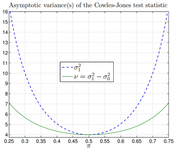
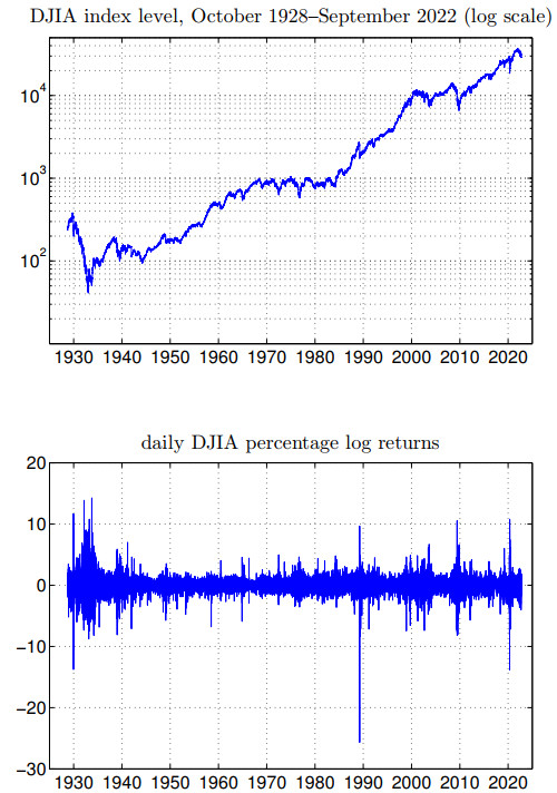
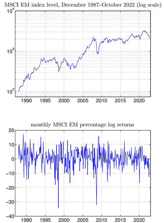
The Cowles-Jones test for sign dependence is one of the earliest tests of the random walk hypothesis, which stands at the beginning of modern empirical finance. The test is still discussed in popular textbooks and used in research articles. However, the Cowles-Jones test statistic considered in the literature requires that the upward probability of the market or asset under consideration be specified under the null hypothesis, which is only very rarely possible. If the upward probability is estimated in advance, the resulting test is undersized (even asymptotically). This note considers a corrected Cowles-Jones test statistic which does not require the upward probability to be specified under the null. It turns out that the asymptotic variance is greatly simplified as compared to the uncorrected test. The corrected test is illustrated with an application to daily returns of the Dow Jones Industrial Average index and monthly returns of the MSCI Emerging Markets index. It is shown that the corrected and uncorrected tests can lead to opposite conclusions.

| [1] | Anderson, TW (1971) The Statistical Analysis of Time Series. John Wiley & Sons, New York. |
| [2] |
Brock W, Lakonishok J, LeBaron, B (1992) Simple Technical Trading Rules and the Stochastic Properties of Stock Returns. J Financ 47: 1731–1764. https://doi.org/10.2307/2328994 doi: 10.2307/2328994

|
| [3] | Campbell JY, Lo AW, MacKinlay AC (1997) The Econometrics of Financial Markets. Princeton University Press, Princeton. |
| [4] |
Charles A, Darné O (2009) Variance ratio test of random walk: an overview. J Econ Surv 23: 503–527. https://doi.org/10.1111/j.1467-6419.2008.00570.x doi: 10.1111/j.1467-6419.2008.00570.x
|
| [5] |
Christoffersen PF, Diebold FX (2006) Financial Asset Returns, Direction-of-Change Forecasting, and Volatility Dynamics. Manage Sci 52: 1273–1287. https://doi.org/10.1287/mnsc.1060.0520 doi: 10.1287/mnsc.1060.0520
|
| [6] |
Cowles A, Jones HE (1937) Some A Posteriori Probabilities in Stock Market Action. Econometrica 5: 280–294. https://doi.org/10.2307/1905515 doi: 10.2307/1905515
|
| [7] | Fiorenzani S, Ravelli S, Edoli E (2012). Handbook of Energy Trading. John Wiley & Sons, Chichester. |
| [8] |
Fisher RA (1925) Theory of Statistical Estimation. Math Proc Cambridge 22: 700–725. https://doi.org/10.1017/S0305004100009580 doi: 10.1017/S0305004100009580
|
| [9] | Haas M, Pigorsch C (2009) Financial Economics: Fat–tailed Distributions. In Meyers, B., editor, Encyclopedia of Complexity and Systems Science. 4. Springer. https://doi.org/10.1007/978-0-387-30440-3 |
| [10] |
Hausman JA (1978) Specification Tests in Econometrics. Econometrica 46: 1251–1271. Specification Tests in Econometrics. https://doi.org/10.2307/1913827 doi: 10.2307/1913827
|
| [11] | Lehmann EL, Casella G (1998) Theory of Point Estimation. Springer, New York. |
| [12] |
Li A, Wei Q, Shi Y, et al. (2023) Research on stock price prediction from a data fusion perspective. Data Sci Financ Econ 3: 230–250. https://doi.org/10.3934/DSFE.2023014 doi: 10.3934/DSFE.2023014
|
| [13] | Linton O (2019) Financial Econometrics: Models and Methods. Cambridge University Press, Cambridge. |
| [14] |
Lo AW (2000) Finance: A Selective Survey. J Am Stat Assoc 95: 629–635. https://doi.org/10.2307/2669406 doi: 10.2307/2669406
|
| [15] |
Mikosch T, Stǎricǎ C (2000) Limit Theory for the Sample Autocorrelations and Extremes of a GARCH (1, 1) Process. Ann Stat 28: 1427–1451. https://doi.org/10.1214/aos/1015957401 doi: 10.1214/aos/1015957401
|
| [16] |
Sullivan R, Timmermann A, White H (1999) Data-Snooping, Technical Trading Rule Performance, and the Bootstrap. J Financ 54: 1647–1691. https://doi.org/10.1111/0022-1082.00163 doi: 10.1111/0022-1082.00163
|
| [17] | Taylor SJ (2005) Asset price Dynamics, Volatility, and Prediction. Princeton University Press, Princeton. |
| [18] | Tsinaslanidis P, Guijarro F (2023) Testing for Sequences and Reversals on Bitcoin Series. In Tsounis, N. and Vlachvei, A., editors, Advances in Empirical Economic Research. ICOAE 2022. Springer, Cham. https://doi.org/10.1007/978-3-031-22749-3 |
| [19] | Williamson SH (2023) Daily Closing Values of the DJA in the United States, 1885 to Present. MeasuringWorth. http://www.measuringworth.com/DJA/ (last accessed: May 5, 2023). |
| [20] |
Xie H, Sun Y, Fan P (2023) Return direction forecasting: a conditional autoregressive shape model with beta density. Financ Innov 9: 1–16. https://doi.org/10.1186/s40854-023-00489-z doi: 10.1186/s40854-023-00489-z
|
Figures(3) / Tables(2)
Markus Haas. The Cowles–Jones test with unspecified upward market probability[J]. Data Science in Finance and Economics, 2023, 3(4): 324-336. doi: 10.3934/DSFE.2023019


 DownLoad: