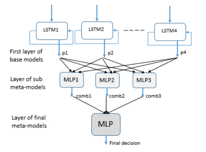
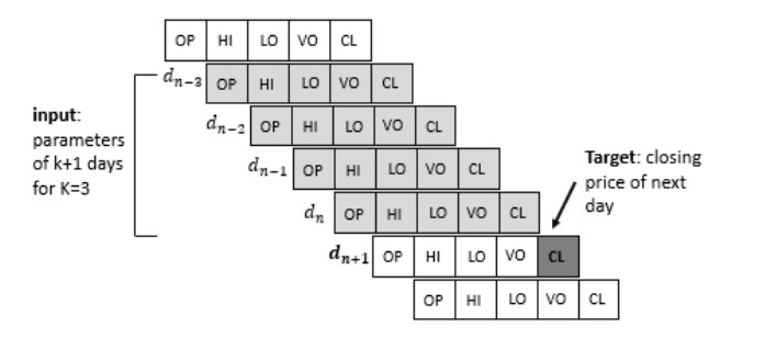
The ability to predict stock-market indices is important to investors and financial decision-makers. However, the uncertainty of available information makes accurate prediction extremely challenging. In this work, we propose and validate a multi-level stacking model of long short-term memory (LSTM) units for the short-term prediction of stock-index closing prices. The proposed machine-learning model is trained using historical data to predict next-day closing prices. The first layer of the multi-level stacked structure contains an ensemble of recurrent LSTM models that receives time-series data of historic opening, closing, high and low prices for current and previous days and outputs predictions about the next day's closing prices. The second and third layers consist of stacked multi-layer perceptron meta-models. We validated the new model on two stock indices, demonstrating its advantages over single-LSTM models. We also compared its performance against several extant statistical and machine-learning models on a subset of Standard & Poor's 500 index data between 2000 and 2016 using correlation and statistical metrics.
Citation: Fatima Tfaily, Mohamad M. Fouad. Multi-level stacking of LSTM recurrent models for predicting stock-market indices[J]. Data Science in Finance and Economics, 2022, 2(2): 147-162. doi: 10.3934/DSFE.2022007
The ability to predict stock-market indices is important to investors and financial decision-makers. However, the uncertainty of available information makes accurate prediction extremely challenging. In this work, we propose and validate a multi-level stacking model of long short-term memory (LSTM) units for the short-term prediction of stock-index closing prices. The proposed machine-learning model is trained using historical data to predict next-day closing prices. The first layer of the multi-level stacked structure contains an ensemble of recurrent LSTM models that receives time-series data of historic opening, closing, high and low prices for current and previous days and outputs predictions about the next day's closing prices. The second and third layers consist of stacked multi-layer perceptron meta-models. We validated the new model on two stock indices, demonstrating its advantages over single-LSTM models. We also compared its performance against several extant statistical and machine-learning models on a subset of Standard & Poor's 500 index data between 2000 and 2016 using correlation and statistical metrics.

| [1] | Al-Hajj R, Assi A, Fouad MM (2018) Forecasting Solar Radiation Strength Using Machine Learning Ensemble. In: 7th International Conference on Renewable Energy Research and Applications (ICRERA), Paris - France, 10: 184-188. IEEE. https://doi.org/10.1109/ICRERA.2018.8567020 |
| [2] | Al-Hajj R, Assi A, Fouad MM (2019) Stacking-Based Ensemble of Support Vector Regressors for One-Day Ahead Solar Irradiance Prediction. In: 8th International Conference on Renewable Energy Research and Applications (ICRERA), Brasov-Romania, 9: 428-433. IEEE. https://doi.org/10.1109/ICRERA47325.2019.8996629 |
| [3] |
Bahrammirzaee A (2010) A comparative survey of artificial intelligence applications in finance: artificial neural networks, expert system and hybrid intelligent systems. Neural Comput Appl 19: 1165-1195. https://doi.org/10.1007/s00521-010-0362-z doi: 10.1007/s00521-010-0362-z

|
| [4] |
Banerjee S, Mukherjee D (2020) Short Term Stock Price Prediction in Indian Market: A Neural Network Perspective. Stud Microeconomics 10: 23-49. https://doi.org/10.1177/2321022220980537 doi: 10.1177/2321022220980537
|
| [5] | Bergstra J, Bengio Y (2012) Random search for hyper-parameter optimization. J Mach Learni Res 13: 281-305. |
| [6] |
Briscoe E, Feldman J (2011) Conceptual complexity and the bias/variance tradeoff. Cognition 118: 2-16. https://doi.org/10.1016/j.cognition.2010.10.004 doi: 10.1016/j.cognition.2010.10.004
|
| [7] |
Cervelló-Royo R, Guijarro F, Michniuk K (2015) Stock market trading rule based on pattern recognition and technical analysis: Forecasting the DJIA index with intraday data. Expert Syst Appl 42: 5963-5975. https://doi.org/10.1016/j.eswa.2015.03.017 doi: 10.1016/j.eswa.2015.03.017
|
| [8] |
Chen Y, Hao Y (2017) A feature weighted support vector machine and K-nearest neighbor algorithm for stock market indices prediction. Expert Syst Appl 80: 340-355. https://doi.org/10.1016/j.eswa.2017.02.044 doi: 10.1016/j.eswa.2017.02.044
|
| [9] | Dietterich TG (2000) Ensemble methods in machine learning. In: Proc. of International workshop on multiple classifier systems-Springer, Cagliari-Italy, 6: 1-15. https://doi.org/10.1007/3-540-45014-9_1 |
| [10] | Gao T, Chai Y, Liu Y (2017) Applying long short term momory neural networks for predicting stock closing price. In: 8th IEEE International Conference on Software Engineering and Service Science (ICSESS), Beijing - China, 12: 575-578. IEEE. https://doi.org/10.1109/ICSESS.2017.8342981 |
| [11] |
Hassan EE, Zhang D (2021) The usage of logistic regression and artificial neural networks for evaluation and predicting property-liability insurers' solvency in Egypt. Data Sci Financ Econ 1: 215-234. https://doi.org/10.3934/DSFE.2021012 doi: 10.3934/DSFE.2021012
|
| [12] | Haykin S (2011) Neural Networks and Learning Machines: a comprehensive foundation. Pearson, 2011. |
| [13] |
Heaton JB, Polson NG, Witte JH (2017) Deep learning for finance: Deep portfolios. Appl Stochastic Models Bus Ind 33: 3-12. https://doi.org/10.1002/asmb.2209 doi: 10.1002/asmb.2209
|
| [14] | Hochreiter S, Schmidhuber J (1997) Long short-term memory. Neural Comput 9: 1735-1780. |
| [15] |
Jiao Y, Jakubowicz J (2017) Predicting stock movement direction with machine learning: An extensive study on S & P 500 stocks. In IEEE International Conference on Big Data (Big Data). 4705-4713. IEEE. https://doi.org/10.1109/BigData.2017.8258518 doi: 10.1109/BigData.2017.8258518
|
| [16] |
Li Y, Yi J, Chen H, et al. (2021) Theory and application of artificial intelligence in financial industry. Data Sci Financ Econ 1: 96-116. https://doi.org/10.3934/DSFE.2021006 doi: 10.3934/DSFE.2021006
|
| [17] |
Liu H, Huang S, Wang P, et al. (2021). A review of data mining methods in financial markets. Data Sci Financ Econ 1: 362-392. https://doi.org/10.3934/DSFE.2021020 doi: 10.3934/DSFE.2021020
|
| [18] |
Lu CJ (2013) Hybridizing nonlinear independent component analysis and support vector regression with particle swarm optimization for stock index forecasting. Neural Comput Appl 23: 2417-2427. https://doi.org/10.1007/s00521-012-1198-5 doi: 10.1007/s00521-012-1198-5
|
| [19] | Pedregosa F, Varoquaux G, Gramfort A, et al. (2011) Scikit-learn: Machine learning in Python. J Mach Learn Res 12: 2825-2830. |
| [20] |
Ren Y, Suganthan PN, Srikanth N (2015) Ensemble methods for wind and solar power forecasting-A state-of-the-art review. Renew Sust Energ Rev 50: 82-91. https://doi.org/10.1016/j.rser.2015.04.081 doi: 10.1016/j.rser.2015.04.081
|
| [21] |
Ren Y, Zhang L, Suganthan PN (2016) Ensemble classification and regression-recent developments, applications and future directions. IEEE Comput Intell Mag 11: 41-53. https://doi.org/10.1109/MCI.2015.2471235 doi: 10.1109/MCI.2015.2471235
|
| [22] | Sagi O, Rokach L (2018) Ensemble learning: A survey. Wiley Interdisciplinary Reviews: Data Mining and Knowledge Discovery 8: 1249. |
| [23] | Vargas M, De Lima B, Evsukoff A (2017) Deep learning for stock market prediction from financial news articles. In: IEEE International Conference on Computational Intelligence and Virtual Environments for Measurement Systems and Applications (CIVEMSA), Annecy-France: 60-65. https://doi.org/10.1109/CIVEMSA.2017.7995302 |
| [24] |
Wang Y, Yan G (2021) Survey on the application of deep learning in algorithmic trading. Data Sci Financ Econ 1: 345-61. https://doi.org/10.3934/DSFE.2021019 doi: 10.3934/DSFE.2021019
|
| [25] |
Weng B, Lu L, Wang X, et al. (2018) Predicting short-term stock prices using ensemble methods and online data sources. Expert Syst Appl 112: 258-273. https://doi.org/10.1016/j.eswa.2018.06.016 doi: 10.1016/j.eswa.2018.06.016
|
| [26] |
Zhong X, Enke D (2017) Forecasting daily stock market return using dimensionality reduction. Expert Syst Appl 67:126-139. https://doi.org/10.1016/j.eswa.2016.09.027 doi: 10.1016/j.eswa.2016.09.027
|
| [27] | Zhang C, Ma Y (2012) Ensemble machine learning: methods and applications. Boston, MA: Springer Science & Business Media. |
Figures(7) / Tables(3)
Fatima Tfaily, Mohamad M. Fouad. Multi-level stacking of LSTM recurrent models for predicting stock-market indices[J]. Data Science in Finance and Economics, 2022, 2(2): 147-162. doi: 10.3934/DSFE.2022007


 DownLoad: