Toxicological considerations of nano-sized plastics

PA Stapleton; PA Stapleton

doi:10.3934/environsci.2019.5.367

AIMS Environmental Science

2019, Volume 6, Issue 5: 367-378. doi: 10.3934/environsci.2019.5.367

Previous Article Next Article

Mini review Special Issues

Toxicological considerations of nano-sized plastics

PA Stapleton ^{1,2
,
,}

1.
Department of Pharmacology and Toxicology, Ernest Mario School of Pharmacy, Rutgers University, 160 Frelinghuysen Rd., Piscataway, NJ 08854, USA
2.
Environmental and Occupational Health Sciences Institute, 170 Frelinghuysen Rd., Piscataway, NJ 08854, USA

Received: 12 July 2019 Accepted: 25 September 2019 Published: 22 October 2019

Undoubtedly, plastics have changed human existence. These pervasive products are used in nearly every field to include technological, biomedical, and domestic applications. Post-consumer plastic waste disposal leading to plastic pollution in landfills, waterways, and oceans represents a worldwide environmental challenge. Accumulation and continued material fragmentation from micro- to nanoplastics has identified concerns pertaining to environmental and human exposures and toxicity. While many studies have focused on particle fate and identification, the toxicological considerations must focus on the biological relevance of particle deposition within a particular organism, compartment, organ, and tissue. Further, concerns exist regarding the physical and chemical properties of the plastic particles during their production and/or degradation. In this minireview we will discuss (1) particle characterization and assessment, (2) environmental concerns, and (3) human toxicity.
- toxicology,
- exposure,
- nanoplastics,
- microplastics
Citation: PA Stapleton. Toxicological considerations of nano-sized plastics[J]. AIMS Environmental Science, 2019, 6(5): 367-378. doi: 10.3934/environsci.2019.5.367

Related Papers:

Abstract

Undoubtedly, plastics have changed human existence. These pervasive products are used in nearly every field to include technological, biomedical, and domestic applications. Post-consumer plastic waste disposal leading to plastic pollution in landfills, waterways, and oceans represents a worldwide environmental challenge. Accumulation and continued material fragmentation from micro- to nanoplastics has identified concerns pertaining to environmental and human exposures and toxicity. While many studies have focused on particle fate and identification, the toxicological considerations must focus on the biological relevance of particle deposition within a particular organism, compartment, organ, and tissue. Further, concerns exist regarding the physical and chemical properties of the plastic particles during their production and/or degradation. In this minireview we will discuss (1) particle characterization and assessment, (2) environmental concerns, and (3) human toxicity.

References

[1]	Nanoplastic should be better understood. (2019) Nat Nanotechnol 14: 299.
[2]	Tsuru T, Shibutani Y (2006) Coupled simulation synchronized by molecular and dislocation dynamics. Comput Methods, Pts 1 and 2: 583-588.
[3]	Gigault J, Halle AT, Baudrimont M, et al. (2018) Current opinion: What is a nanoplastic? Environ Pollut 235: 1030-1034. doi: 10.1016/j.envpol.2018.01.024
[4]	Jahnke A, Arp HPH, Escher BI, et al. (2017) Reducing Uncertainty and Confronting Ignorance about the Possible Impacts of Weathering Plastic in the Marine Environment. Environ Sci Tech Lett 4: 85-90. doi: 10.1021/acs.estlett.7b00008
[5]	Miernicki M, Hofmann T, Eisenberger I, et al. (2019) Legal and practical challenges in classifying nanomaterials according to regulatory definitions. Nat Nanotechnol 14: 208-216. doi: 10.1038/s41565-019-0396-z
[6]	Oberdorster G, Oberdorster E, Oberdorster J (2005) Nanotoxicology: an emerging discipline evolving from studies of ultrafine particles. Environ Health Persp 113: 823-839. doi: 10.1289/ehp.7339
[7]	Wagner S, Reemtsma T (2019) Things we know and don't know about nanoplastic in the environment. Nat Nanotechnol 14: 300-301. doi: 10.1038/s41565-019-0424-z
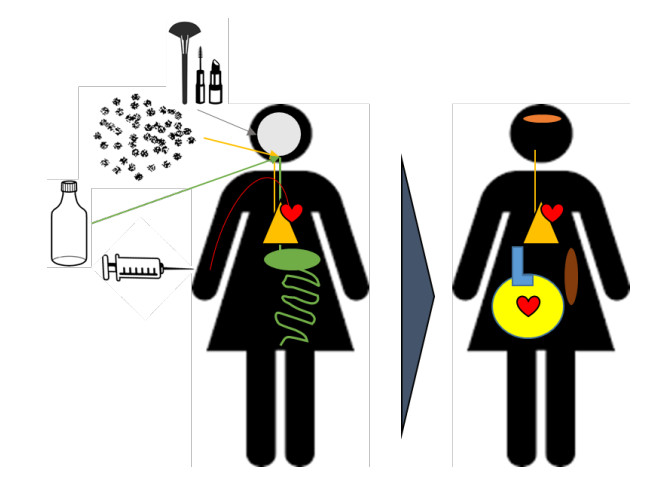
[8]	Stapleton PA. Nanoplastic translocation between the maternal-fetal environment 2019; Rutgers University, New Brunswick, NJ.
[9]	Sander M, Kohler HE, McNeill K (2019) Assessing the environmental transformation of nanoplastic through (13)C-labelled polymers. Nat Nanotechnol 14: 301-303. doi: 10.1038/s41565-019-0420-3
[10]	Mitrano DM, Beltzung A, Frehland S, et al. (2019) Synthesis of metal-doped nanoplastics and their utility to investigate fate and behaviour in complex environmental systems. Nat Nanotechnol 14: 362-368. doi: 10.1038/s41565-018-0360-3
[11]	Silva AB, Bastos AS, Justino CIL, et al. (2018) Microplastics in the environment: Challenges in analytical chemistry-A review. Anal Chim Acta 1017: 1-19. doi: 10.1016/j.aca.2018.02.043
[12]	Song YK, Hong SH, Jang M, et al. (2015) A comparison of microscopic and spectroscopic identification methods for analysis of microplastics in environmental samples. Mar Pollut Bull 93: 202-209. doi: 10.1016/j.marpolbul.2015.01.015
[13]	Bouwmeester H, Hollman PC, Peters RJ (2015) Potential Health Impact of Environmentally Released Micro-and Nanoplastics in the Human Food Production Chain: Experiences from Nanotoxicology. Environ Sci Technol 49: 8932-8947. doi: 10.1021/acs.est.5b01090
[14]	Council RD Different Types of Plastic and Their Classification. https://www.ryedale.gov.uk/attachments/article/690/Different_plastic_polymer_types.pdf.
[15]	Oehlmann J, Schulte-Oehlmann U, Kloas W, et al. (2009) A critical analysis of the biological impacts of plasticizers on wildlife. Philos Trans R Soc Lond B Biol Sci 364: 2047-2062. doi: 10.1098/rstb.2008.0242
[16]	Song Z, Yang X, Chen F, et al. (2019) Fate and transport of nanoplastics in complex natural aquifer media: Effect of particle size and surface functionalization. Sci Total Environ 669: 120-128. doi: 10.1016/j.scitotenv.2019.03.102
[17]	Liu L, Fokkink R, Koelmans AA (2016) Sorption of polycyclic aromatic hydrocarbons to polystyrene nanoplastic. Environ Toxicol Chem 35: 1650-1655. doi: 10.1002/etc.3311
[18]	Tallec K, Blard O, Gonzalez-Fernandez C, et al. (2019) Surface functionalization determines behavior of nanoplastic solutions in model aquatic environments. Chemosphere 225: 639-646. doi: 10.1016/j.chemosphere.2019.03.077
[19]	Alimi OS, Farner Budarz J, Hernandez LM, et al. (2018) Microplastics and Nanoplastics in Aquatic Environments: Aggregation, Deposition, and Enhanced Contaminant Transport. Environ Sci Technol 52: 1704-1724. doi: 10.1021/acs.est.7b05559
[20]	Bhattacharjee S, Ershov D, Islam MA, et al. (2014) Role of membrane disturbance and oxidative stress in the mode of action underlying the toxicity of differently charged polystyrene nanoparticles. Rsc Adv 4: 19321-19330. doi: 10.1039/C3RA46869K
[21]	Cedervall T, Hansson LA, Lard M, et al. (2012) Food chain transport of nanoparticles affects behaviour and fat metabolism in fish. PLoS One 7: e32254. doi: 10.1371/journal.pone.0032254
[22]	Ng EL, Huerta Lwanga E, Eldridge SM, et al. (2018) An overview of microplastic and nanoplastic pollution in agroecosystems. Sci Total Environ 627: 1377-1388. doi: 10.1016/j.scitotenv.2018.01.341
[23]	Bhargava S, Lee SSC, Ying LSM, et al. (2018) Fate of Nanoplastics in Marine Larvae: A Case Study Using Barnacles, Amphibalanus amphitrite. Acs Sustainable Chem& Engin 6: 6932-6940.
[24]	Chang CW, Seibel AJ, Song JW (2019) Application of microscale culture technologies for studying lymphatic vessel biology. Microcirculat e12547.
[25]	Della Torre C, Bergami E, Salvati A, et al. (2014) Accumulation and Embryotoxicity of Polystyrene Nanoparticles at Early Stage of Development of Sea Urchin Embryos Paracentrotus lividus. Environ Sci & Techno 48: 12302-12311.
[26]	Canesi L, Ciacci C, Fabbri R, et al. (2016) Interactions of cationic polystyrene nanoparticles with marine bivalve hemocytes in a physiological environment: Role of soluble hemolymph proteins. Environ Res 150: 73-81. doi: 10.1016/j.envres.2016.05.045
[27]	Shao H, Han Z, Krasteva N, et al. (2019) Identification of signaling cascade in the insulin signaling pathway in response to nanopolystyrene particles. Nanotoxicology 13: 174-188. doi: 10.1080/17435390.2018.1530395
[28]	Mishra P, Vinayagam S, Duraisamy K, et al. (2019) Distinctive impact of polystyrene nano-spherules as an emergent pollutant toward the environment. Environ Sci Pollut Res Int 26: 1537-1547. doi: 10.1007/s11356-018-3698-z
[29]	Fu SF, Ding JN, Zhang Y, et al. (2018) Exposure to polystyrene nanoplastic leads to inhibition of anaerobic digestion system. Sci Total Environ 625: 64-70. doi: 10.1016/j.scitotenv.2017.12.158
[30]	Zhang W, Liu Z, Tang S, et al. (2019) Transcriptional response provides insights into the effect of chronic polystyrene nanoplastic exposure on Daphnia pulex. Chemosphere 238: 124563.
[31]	Greven AC, Merk T, Karagoz F, et al. (2016) Polycarbonate and polystyrene nanoplastic particles act as stressors to the innate immune system of fathead minnow (Pimephales promelas). Environ Toxicol Chem 35: 3093-3100. doi: 10.1002/etc.3501
[32]	Shen M, Zhang Y, Zhu Y, et al. (2019) Recent advances in toxicological research of nanoplastics in the environment: A review. Environ Pollut 252: 511-521. doi: 10.1016/j.envpol.2019.05.102
[33]	Hernandez LMY, N.; Tufenkji, N. (2017) Are there nanoplastics in you personal care products. Environ Sci Technol Lett 4: 280-285. doi: 10.1021/acs.estlett.7b00187
[34]	Mason SA, Welch VG, Neratko J (2018) Synthetic Polymer Contamination in Bottled Water. Front Chem 6: 407. doi: 10.3389/fchem.2018.00407
[35]	Dris R, Gasperi J, Mirande C, et al. (2017) A first overview of textile fibers, including microplastics, in indoor and outdoor environments. Environ Pollut 221: 453-458. doi: 10.1016/j.envpol.2016.12.013
[36]	Prata JC (2018) Airborne microplastics: Consequences to human health? Environ Pollut 234: 115-126. doi: 10.1016/j.envpol.2017.11.043
[37]	Toussaint B, Raffael B, Angers-Loustau A, et al. (2019) Review of micro- and nanoplastic contamination in the food chain. Food Addit Contam Part A Chem Anal Control Expo Risk Assess 36: 639-673. doi: 10.1080/19440049.2019.1583381
[38]	Cox KD, Covernton GA, Davies HL, et al. (2019) Human Consumption of Microplastics. Environ Sci Technol 53: 7068-7074. doi: 10.1021/acs.est.9b01517
[39]	Lehner R, Weder C, Petri-Fink A, et al. (2019) Emergence of Nanoplastic in the Environment and Possible Impact on Human Health. Environ Sci Technol 53: 1748-1765. doi: 10.1021/acs.est.8b05512
[40]	Schwabl P, Liebmann B, Koppel S, et al. (2018) Assessment of microplastic concentrations in human stool-Preliminary results of a prospective study. United European Gastroenterol J 6: A127.
[41]	Brook RD, Brook JR, Rajagopalan S (2003) Air pollution: the "Heart" of the problem. Curr Hypertens Rep 5: 32-39. doi: 10.1007/s11906-003-0008-y
[42]	Ohlwein S, Kappeler R, Kutlar Joss M, et al. (2019) Health effects of ultrafine particles: a systematic literature review update of epidemiological evidence. Int J Public Health 64: 547-559. doi: 10.1007/s00038-019-01202-7
[43]	Stapleton PA, Minarchick VC, McCawley M, et al. (2012) Xenobiotic particle exposure and microvascular endpoints: a call to arms. Microcirculation 19: 126-142. doi: 10.1111/j.1549-8719.2011.00137.x
[44]	Stapleton PA, Minarchick VC, Cumpston AM, et al. (2012) Impairment of coronary arteriolar endothelium-dependent dilation after multi-walled carbon nanotube inhalation: a time-course study. Int J Mol Sci 13: 13781-13803. doi: 10.3390/ijms131113781
[45]	Porter DW, Hubbs AF, Mercer RR, et al. (2010) Mouse pulmonary dose- and time course-responses induced by exposure to multi-walled carbon nanotubes. Toxicology 269: 136-147. doi: 10.1016/j.tox.2009.10.017
[46]	Mastrangelo G, Fedeli U, Fadda E, et al. (2002) Epidemiologic evidence of cancer risk in textile industry workers: a review and update. Toxicol Ind Health 18: 171-181. doi: 10.1191/0748233702th139rr
[47]	Porter DW, Castranova V, Robinson VA, et al. (1999) Acute inflammatory reaction in rats after intratracheal instillation of material collected from a nylon flocking plant. J Toxicol Environ Health A 57: 25-45. doi: 10.1080/009841099157845
[48]	D'Errico JN, Fournier SB, Stapleton PA (2019) Ex vivo perfusion of the rodent placenta. J Vis Exp: e59412.
[49]	Som C, Wick P, Krug H, et al. (2011) Environmental and health effects of nanomaterials in nanotextiles and facade coatings. Environ Int 37: 1131-1142. doi: 10.1016/j.envint.2011.02.013
[50]	Lim SL, Ng CT, Zou L, et al. (2019) Targeted metabolomics reveals differential biological effects of nanoplastics and nanoZnO in human lung cells. Nanotoxicology: 1-34.
[51]	Schirinzi GF, Perez-Pomeda I, Sanchis J, et al. (2017) Cytotoxic effects of commonly used nanomaterials and microplastics on cerebral and epithelial human cells. Environ Res 159: 579-587. doi: 10.1016/j.envres.2017.08.043
[52]	Forte M, Iachetta G, Tussellino M, et al. (2016) Polystyrene nanoparticles internalization in human gastric adenocarcinoma cells. Toxicol In Vitro 31: 126-136. doi: 10.1016/j.tiv.2015.11.006
[53]	Parenti CC, Ghilardi A, Della Torre C, et al. (2019) Evaluation of the infiltration of polystyrene nanobeads in zebrafish embryo tissues after short-term exposure and the related biochemical and behavioural effects. Environ Pollut 254: 112947. doi: 10.1016/j.envpol.2019.07.115
[54]	Grafmueller S, Manser P, Diener L, et al. (2015) Transfer studies of polystyrene nanoparticles in the ex vivo human placenta perfusion model: key sources of artifacts. Sci Technol Adv Mater 16: 044602. doi: 10.1088/1468-6996/16/4/044602
[55]	Grafmueller S, Manser P, Diener L, et al. (2015) Bidirectional Transfer Study of Polystyrene Nanoparticles across the Placental Barrier in an ex Vivo Human Placental Perfusion Model. Environ Health Perspect 123: 1280-1286. doi: 10.1289/ehp.1409271
[56]	Vogel SA (2009) The politics of plastics: the making and unmaking of bisphenol a "safety". Am J Public Health 99 Suppl 3: S559-566.
[57]	Moon MK (2019) Concern about the Safety of Bisphenol A Substitutes. Diabetes Metab J 43: 46-48. doi: 10.4093/dmj.2019.0027
[58]	Liu B, Lehmler HJ, Sun Y, et al. (2019) Association of Bisphenol A and Its Substitutes, Bisphenol F and Bisphenol S, with Obesity in United States Children and Adolescents. Diabetes Metab J 43: 59-75. doi: 10.4093/dmj.2018.0045
[59]	Liu B, Lehmler HJ, Sun Y, et al. (2017) Bisphenol A substitutes and obesity in US adults: analysis of a population-based, cross-sectional study. Lancet Planet Health 1: e114-e122. doi: 10.1016/S2542-5196(17)30049-9
[60]	Pelch K, Wignall JA, Goldstone AE, et al. (2019) A scoping review of the health and toxicological activity of bisphenol A (BPA) structural analogues and functional alternatives. Toxicology 424: 152235. doi: 10.1016/j.tox.2019.06.006
[61]	Siracusa JS, Yin L, Measel E, et al. (2018) Effects of bisphenol A and its analogs on reproductive health: A mini review. Reprod Toxicol 79: 96-123. doi: 10.1016/j.reprotox.2018.06.005
[62]	Usman A, Ikhlas S, Ahmad M (2019) Occurrence, toxicity and endocrine disrupting potential of Bisphenol-B and Bisphenol-F: A mini-review. Toxicol Lett 312: 222-227. doi: 10.1016/j.toxlet.2019.05.018

Reader Comments

Your name:*

Email:*
© 2019 the Author(s), licensee AIMS Press. This is an open access article distributed under the terms of the Creative Commons Attribution License (http://creativecommons.org/licenses/by/4.0)