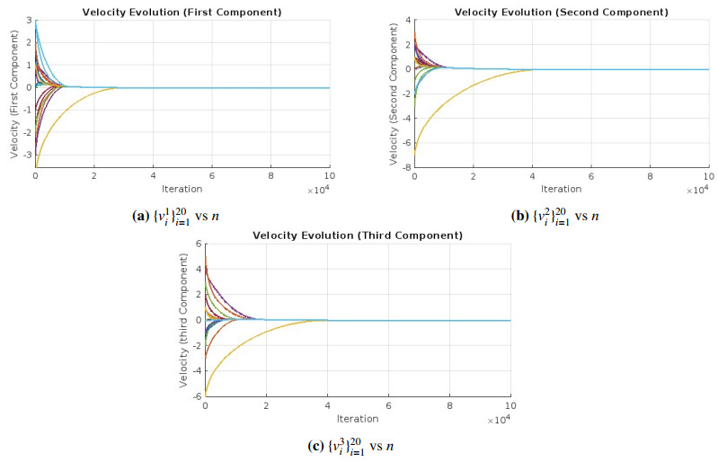
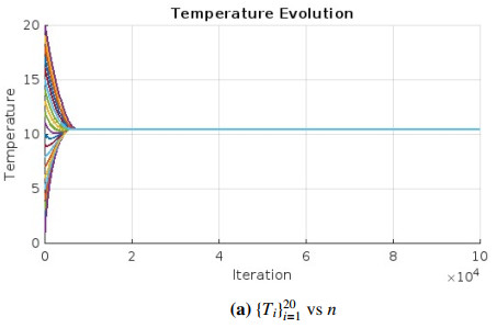
We illustrate finite-in-time flocking in the thermodynamic Cucker–Smale (TCS) model. First, we extend the original TCS model to allow for a continuous vector field with a locally Lipschitz continuity. Then, within this system, we derive appropriate dissipative inequalities concerning the position-velocity-temperature using several preparatory estimates. Subsequently, based on initial data and system parameters, we formulate sufficient conditions to guarantee the desired finite-time flocking in each case where the communication weight conditions are divided into two scenarios: one with a positive lower bound and another with nonnegativity and monotonicity. Finally, we provide several numerical simulations and compare them with the analytical results.
Citation: Hyunjin Ahn, Se Eun Noh. Finite-in-time flocking of the thermodynamic Cucker–Smale model[J]. Networks and Heterogeneous Media, 2024, 19(2): 526-546. doi: 10.3934/nhm.2024023
We illustrate finite-in-time flocking in the thermodynamic Cucker–Smale (TCS) model. First, we extend the original TCS model to allow for a continuous vector field with a locally Lipschitz continuity. Then, within this system, we derive appropriate dissipative inequalities concerning the position-velocity-temperature using several preparatory estimates. Subsequently, based on initial data and system parameters, we formulate sufficient conditions to guarantee the desired finite-time flocking in each case where the communication weight conditions are divided into two scenarios: one with a positive lower bound and another with nonnegativity and monotonicity. Finally, we provide several numerical simulations and compare them with the analytical results.

| [1] |
H. Ahn, Emergent behaviors of thermodynamic Cucker–Smale ensemble with a unit-speed constraint, Discrete Continuous Dyn Syst Ser B, 28 (2023), 4800–4825. https://doi.org/10.3934/dcdsb.2023042 doi: 10.3934/dcdsb.2023042

|
| [2] |
H. Ahn, Uniform stability of Cucker–Smale and thermodynamic Cucker–Smale ensembles with singular kernels, Netw. Heterog. Media, 17 (2022), 753–782. https://doi.org/10.3934/nhm.2022025 doi: 10.3934/nhm.2022025
|
| [3] |
H. Ahn, S. Y. Ha, W. Shim, Emergent behaviors of the discrete thermodynamic Cucker–Smale model on Riemannian manifolds, J. Math. Phys., 62 (2021), 122701. https://doi.org/10.1063/5.0058616 doi: 10.1063/5.0058616
|
| [4] |
H. Ahn, S. Y. Ha, W. Shim, Emergent dynamics of a thermodynamic Cucker–Smale ensemble on complete Riemannian manifolds, Kinet. Relat. Models., 14 (2021), 323–351. https://doi.org/10.3934/krm.2021007 doi: 10.3934/krm.2021007
|
| [5] |
J. A. Carrillo, Y. P. Choi, P. B. Muncha, J. Peszek, Sharp conditions to avoid collisions in singular Cucker–Smale interactions, Nonlinear Anal Real World Appl, 37 (2017), 317–328. https://doi.org/10.1016/j.nonrwa.2017.02.017 doi: 10.1016/j.nonrwa.2017.02.017
|
| [6] |
J. A. Carrillo, M. Fornasier, J. Rosado, G. Toscani, Asymptotic flocking dynamics for the kinetic Cucker–Smale model, SIAM. J. Math. Anal., 42 (2010), 218–236. https://doi.org/https://doi.org/10.1137/090757290 doi: 10.1137/090757290
|
| [7] |
P. Cattiaux, F. Delebecque, L. Pedeches, Stochastic Cucker–Smale models: old and new, Ann. Appl. Probab., 28 (2018), 3239–3286. https://doi.org/10.1214/18-AAP1400 doi: 10.1214/18-AAP1400
|
| [8] |
H. Cho, J. G. Dong, S. Y. Ha, Emergent behaviors of a thermodynamic Cucker–Smale flock with a time-delay on a general digraph, Math. Methods Appl. Sci., 45 (2021), 164–196. https://doi.org/https://doi.org/10.1002/mma.7771 doi: 10.1002/mma.7771
|
| [9] |
S. H. Choi, S. Y. Ha, Emergence of flocking for a multi-agent system moving with constant speed, Commun. Math. Sci., 14 (2016), 953–972. https://doi.org/10.4310/CMS.2016.v14.n4.a4 doi: 10.4310/CMS.2016.v14.n4.a4
|
| [10] |
Y. P. Choi, S. Y. Ha, J. Kim, Propagation of regularity and finite-time collisions for the thermomechanical Cucker–Smale model with a singular communication, Netw. Heterog. Media, 13 (2018), 379–407. https://doi.org/10.3934/nhm.2018017 doi: 10.3934/nhm.2018017
|
| [11] |
Y. P. Choi, D. Kalise, J. Peszek, A. A Peters, A collisionless singular Cucker–Smale model with decentralized formation control, SIAM J. Appl. Dyn. Syst., 18 (2019), 1954–1981. https://doi.org/10.1137/19M1241799 doi: 10.1137/19M1241799
|
| [12] |
J. Cho, S. Y. Ha, F. Huang, C. Jin, D. Ko, Emergence of bi-cluster flocking for the Cucker–Smale model, Math. Models Methods Appl. Sci., 26 (2016), 1191–1218. https://doi.org/10.1142/S0218202516500287 doi: 10.1142/S0218202516500287
|
| [13] | F. Cucker, J. G. Dong, A conditional, collision-avoiding, model for swarming, Discrete Contin. Dyn. Syst., 34 (2014), 1009–1020. https://doi.org/10.3934/dcds.2014.34.1009 |
| [14] | F. Cucker, S. Smale, Emergent behavior in flocks, IEEE Trans. Automat. Control, 52 (2007), 852–862. https://doi.org/10.1109/TAC.2007.895842 |
| [15] |
J. G. Dong, S. Y. Ha, D. Kim, From discrete Cucker–Smale model to continuous Cucker–Smale model in a temperature field, J. Math. Phys., 60 (2019), 072705. https://doi.org/10.1063/1.5084770 doi: 10.1063/1.5084770
|
| [16] |
J. G. Dong, S. Y. Ha, D. Kim, Emergent behaviors of continuous and discrete thermomechanical Cucker–Smale models on general digraphs, Math. Models Methods Appl. Sci., 29 (2019), 589–632. https://doi.org/10.1142/S0218202519400013 doi: 10.1142/S0218202519400013
|
| [17] |
A. Figalli, M. J. Kang, A rigorous derivation from the kinetic Cucker–Smale model to the pressureless Euler system with nonlocal alignment, Anal. PDE., 12 (2019), 843–866. https://doi.org/10.2140/apde.2019.12.843 doi: 10.2140/apde.2019.12.843
|
| [18] |
S. Y. Ha, J. Jeong, S. E. Noh, Q. Xiao, X. Zhang, Emergent dynamics of Cucker–Smale flocking particles in a random environment, J. Differ. Equ., 262 (2017), 2554–2591. https://doi.org/10.1016/j.jde.2016.11.017 doi: 10.1016/j.jde.2016.11.017
|
| [19] |
S. Y. Ha, M. J. Kang, J. Kim, W. Shim, Hydrodynamic limit of the kinetic thermomechanical Cucker–Smale model in a strong local alignment regime, Commun. Pure Appl. Anal., 19 (2020), 1233–1256. https://doi.org/10.3934/cpaa.2020057 doi: 10.3934/cpaa.2020057
|
| [20] |
S. Y. Ha, D. Kim, J. Lee, S. E. Noh, Emergent dynamics of an orientation flocking model for multi-agent system, Discrete Contin. Dyn. Syst., 40 (2020), 2037–2060. https://doi.org/10.3934/dcds.2020105 doi: 10.3934/dcds.2020105
|
| [21] |
S. Y. Ha, J. Kim, C. Min, T. Ruggeri, X. Zhang, Uniform stability and mean-field limit of a thermodynamic Cucker–Smale model, Quart. Appl. Math., 77 (2019), 131–176. https://doi.org/10.1090/qam/1517 doi: 10.1090/qam/1517
|
| [22] |
S. Y. Ha, J. Kim, T. Ruggeri, Emergent behaviors of thermodynamic Cucker–Smale particles, SIAM J. Math. Anal., 50 (2019), 3092–3121. https://doi.org/10.1137/17M111064 doi: 10.1137/17M111064
|
| [23] |
S. Y. Ha, J. G. Liu, A simple proof of Cucker–Smale flocking dynamics and mean-field limit, Commun. Math. Sci., 7 (2009), 297–325. https://doi.org/10.4310/CMS.2009.v7.n2.a2 doi: 10.4310/CMS.2009.v7.n2.a2
|
| [24] |
S. Y. Ha, T. Ruggeri, Emergent dynamics of a thermodynamically consistent particle model, Arch. Ration. Mech. Anal., 223 (2017), 1397–1425. https://doi.org/10.1007/s00205-016-1062-3 doi: 10.1007/s00205-016-1062-3
|
| [25] |
S. Y. Ha, E. Tadmor, From particle to kinetic and hydrodynamic description of flocking, Kinet. Relat. Models., 1 (2008), 415–435. https://doi.org/10.3934/krm.2008.1.415 doi: 10.3934/krm.2008.1.415
|
| [26] |
H. Gayathri, P. M. Aparna, A. Verma, A review of studies on understanding crowd dynamics in the context of crowd safety in mass religious gatherings, Int. J. Disaster Risk Sci., 25 (2017), 82–91. https://doi.org/10.1016/j.ijdrr.2017.07.017 doi: 10.1016/j.ijdrr.2017.07.017
|
| [27] |
T. K. Karper, A. Mellet, K. Trivisa, Hydrodynamic limit of the kinetic Cucker–Smale flocking model, Math. Models Methods Appl. Sci., 25 (2015), 131–163. https://doi.org/10.1142/S0218202515500050 doi: 10.1142/S0218202515500050
|
| [28] |
T. K. Karper, A. Mellet, K. Trivisa, Existence of weak solutions to kinetic flocking models, SIAM. J. Math. Anal., 45 (2013), 215–243. https://doi.org/10.1137/12086682 doi: 10.1137/12086682
|
| [29] |
Z. Li, X. Xue, Cucker–Smale flocking under rooted leadership with fixed and switching topologies, SIAM J. Appl. Math., 70 (2010), 3156–3174. https://doi.org/10.1137/100791774 doi: 10.1137/100791774
|
| [30] |
P. B. Mucha, J. Peszek, The Cucker–Smale equation: singular communication weight, measure-valued solutions and weak-atomic uniqueness, Arch. Rational Mech. Anal., 227 (2018), 273–308. https://doi.org/10.1007/s00205-017-1160-x doi: 10.1007/s00205-017-1160-x
|
| [31] |
J. Park, H. J. Kim, S. Y. Ha, Cucker–Smale flocking with inter-particle bonding forces, IEEE Trans. Automat. Control, 55 (2010), 2617–2623. https://doi.org/10.1109/TAC.2010.2061070 doi: 10.1109/TAC.2010.2061070
|
| [32] |
L. Perea, G. Gomez, P. Elosegui, Extension of the Cucker–Smale control law to space flight formations, J. Guid. Control, 32 (2009), 527–537. https://doi.org/10.2514/1.36269 doi: 10.2514/1.36269
|
| [33] |
J. Peszek, Discrete Cucker–Smale flocking model with a weakly singular kernel, SIAM J. Math. Anal., 47 (2015), 3671–3686. https://doi.org/10.1137/15M1009299 doi: 10.1137/15M1009299
|
| [34] |
B. Piccoli, F. Rossi, E. Trélat, Control to flocking of the kinetic Cucker–Smale model, SIAM J. Math. Anal., 47 (2014), 4685–4719. https://doi.org/10.1137/140996501 doi: 10.1137/140996501
|
| [35] |
L. Ru, X. Li, Y. Liu, X. Wang, Finite-time flocking of Cucker–Smale model with unknown intrinsic dynamics, Discrete Continuous Dyn Syst Ser B, 28 (2023), 3680–3696. https://doi.org/10.3934/dcdsb.2022237 doi: 10.3934/dcdsb.2022237
|
| [36] |
C. M. Topaz, A. L. Bertozzi, Swarming patterns in a two-dimensional kinematic model for biological groups, SIAM J. Appl. Math., 65 (2004), 152–174. https://doi.org/10.1137/S0036139903437424 doi: 10.1137/S0036139903437424
|
| [37] | Y. Z. Sun, F. Liu, W. Li, H. J. Shi, Finite-time flocking of Cucker–Smale systems, 34th Chinese Control Conference (CCC), (2015), 7016–7020. https://doi.org/10.1109/ChiCC.2015.7260749 |
Figures(2)
Hyunjin Ahn, Se Eun Noh. Finite-in-time flocking of the thermodynamic Cucker–Smale model[J]. Networks and Heterogeneous Media, 2024, 19(2): 526-546. doi: 10.3934/nhm.2024023


 DownLoad: