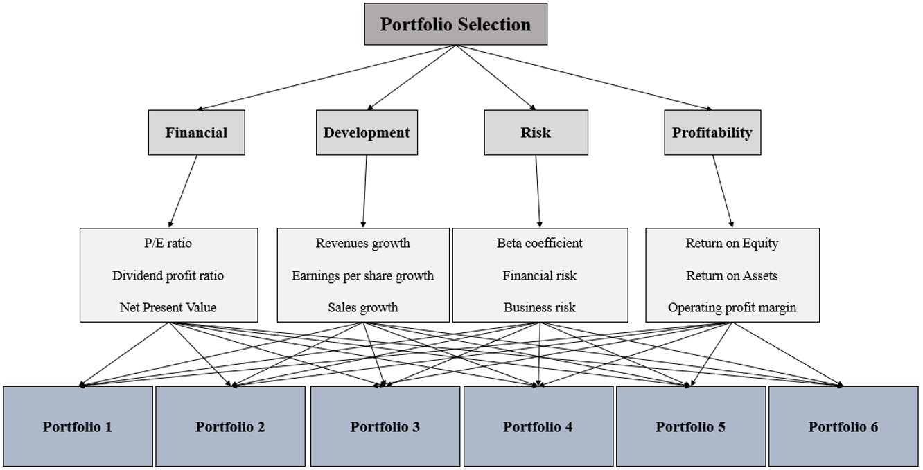
In today's economic world, due to the growth of the capital market, the importance for people to invest has increased. The most important concern for investors is choosing the best portfolio for investment. For complex decisions in which the decision maker is ambiguous, such as portfolio selection, using the multi-criteria decision making (MCDM) technique to prioritize options and decide on the optimal choice is the best solution. In this research, a generalization of this method utilizing the intuitionistic fuzzy analytic hierarchy process (IFAHP) was discussed. Considering the importance of this topic in today's economy, the purpose of this research was to describe and apply the new integrated technique of IFAHP for ranking the portfolio of companies admitted to the Tehran Stock Exchange. For this purpose, using the statistics published by the Tehran Stock Exchange, six companies including Jabra Ben Hayyan, Kaghazsazi Kaveh, Laabiran, Daro Luqman, Pashme Shishe Iran, and Bourse Kala Iran were examined. These companies were the best options for investment according to the charts and indices of the stock exchange at the time of our research. Finally, using the technique mentioned above, we described the evaluation and ranking of portfolios for confident and efficient decision -making.
Citation: Soheila Senfi, Reza Sheikh, Shib Sankar Sana. A portfolio selection using the intuitionistic fuzzy analytic hierarchy process: A case study of the Tehran Stock Exchange[J]. Green Finance, 2024, 6(2): 219-248. doi: 10.3934/GF.2024009
In today's economic world, due to the growth of the capital market, the importance for people to invest has increased. The most important concern for investors is choosing the best portfolio for investment. For complex decisions in which the decision maker is ambiguous, such as portfolio selection, using the multi-criteria decision making (MCDM) technique to prioritize options and decide on the optimal choice is the best solution. In this research, a generalization of this method utilizing the intuitionistic fuzzy analytic hierarchy process (IFAHP) was discussed. Considering the importance of this topic in today's economy, the purpose of this research was to describe and apply the new integrated technique of IFAHP for ranking the portfolio of companies admitted to the Tehran Stock Exchange. For this purpose, using the statistics published by the Tehran Stock Exchange, six companies including Jabra Ben Hayyan, Kaghazsazi Kaveh, Laabiran, Daro Luqman, Pashme Shishe Iran, and Bourse Kala Iran were examined. These companies were the best options for investment according to the charts and indices of the stock exchange at the time of our research. Finally, using the technique mentioned above, we described the evaluation and ranking of portfolios for confident and efficient decision -making.

| [1] |
Ayyildiz E, TaskinGumus A (2021) Interval-valued pythagorean fuzzy AHP method-based supply chain performance evaluation by a new extension of SCOR model: SCOR 4.0. Complex Intell Syst 7: 559–576. https://doi.org/10.1007/s40747-020-00221-9 doi: 10.1007/s40747-020-00221-9

|
| [2] |
Bektur G (2021) A hybrid fuzzy MCDM approach for sustainable project portfolio selection problem and an application for a construction company. Afyon Kocatepe University J Econ Admin Sci 23: 182–194. https://doi.org/10.33707/akuiibfd.911236 doi: 10.33707/akuiibfd.911236
|
| [3] |
Bernal M, Anselmo Alvarez P, Munoz M, et al. (2021) A multicriteria hierarchical approach for portfolio selection in a stock exchange. J Intell Fuzzy Syst 40: 1945–1955. https://doi.org/10.3233/JIFS-189198 doi: 10.3233/JIFS-189198
|
| [4] |
Chen A, Lu Y, Wang B (2017) Customers' purchase decision-making process in social commerce: A social learning perspective. Int J Inf Manag 37: 627–638. https://doi.org/10.1016/j.ijinfomgt.2017.05.001 doi: 10.1016/j.ijinfomgt.2017.05.001
|
| [5] |
Cheng KC, Huang MJ, Fu CK, et al. (2021) Establishing a multiple-criteria decision-making model for stock investment decisions using data mining techniques. Sustainability 13. https://doi.org/10.3390/su13063100 doi: 10.3390/su13063100
|
| [6] | Cohon JL (2004) Multiobjective programming and planning. Mathematics in Science and Engineering, 140, The Johns Hopkins University, Baltimore, Maryland. |
| [7] |
DeMiguel V, Garlappi L, Nogales FJ, et al. (2009) A generalized approach to portfolio optimization: Improving performance by constraining portfolio norms. Manag Sci 55: 798–812. https://doi.org/10.1287/mnsc.1080.0986 doi: 10.1287/mnsc.1080.0986
|
| [8] |
Deng X (2022) Application research and analysis of management accounting in enterprise strategy based on FAHP Model. Adv Econ Bus Manag Res 217: 14. https://doi.org/10.2991/aebmr.k.220502.003 doi: 10.2991/aebmr.k.220502.003
|
| [9] | Elton EJ, Gruber MJ (1995) Modern portfolio theory and invesment analysis (5th ed.). New York: John Wiley and Sons Inc. |
| [10] |
Gupta S, Bandyopadhyay G, Biswas S, et al. (2023) An integrated framework for classification and selection of stocks for portfolio construction: Evidence from NSE, India. Decis Mak Appl Manag Eng 6: 774–803.https://doi.org/10.31181/dmame0318062021g doi: 10.31181/dmame0318062021g
|
| [11] |
Haseli G, Sheikh R, Sana SS (2019) Base-criterion on multi-criteria decision-making method and its applications. Int J Manag Sci Engi Manag 15: 79-88. https://doi.org/10.1080/17509653.2019.1633964 doi: 10.1080/17509653.2019.1633964
|
| [12] |
Ilbahar E, Kahraman C, Cebi S (2022) Risk assessment of renewable energy investments: A modified failure mode and effect analysis based on prospect theory and intuitionistic fuzzy AHP. Int J Energy 239: 121907. https://doi.org/10.1016/j.energy.2021.121907 doi: 10.1016/j.energy.2021.121907
|
| [13] |
Javaherian N, Hamzehee A, SayyadiTooranloo H (2021) Designing an intuitionistic fuzzy network data envelopment analysis model for efficiency evaluation of decision-making units with two-stage structures. Adv Fuzzy Syst 2021: 1–15. https://doi.org/10.1155/2021/8860634 doi: 10.1155/2021/8860634
|
| [14] |
Jin M, Li Z, Yuan S (2021) Research and analysis on Markowitz model and Index Model of portfolio selection. Adv Econ Bus Manag Res 203: 1142–1150. https://doi.org/10.2991/assehr.k.211209.186 doi: 10.2991/assehr.k.211209.186
|
| [15] |
Leung MF, Wang J (2020) Minimax and biobjective portfolio selection based on collaborative neurodynamic optimization. Ieee T Neur Net Lear Syst 32: 2825–2836. https://doi.org/10.1109/TNNLS.2019.2957105 doi: 10.1109/TNNLS.2019.2957105
|
| [16] |
Leung MF, Wang J, Li D (2021) Decentralized robust portfolio optimization based on cooperative-competitive multiagent systems. Ieee T Cybernetics 52: 12785–12794. https://doi.org/10.1109/TCYB.2021.3088884 doi: 10.1109/TCYB.2021.3088884
|
| [17] |
Li B, Wang J, Huang D, et al. (2018) Transaction cost optimization for online portfolio selection. Quant Financ 18: 1411–1424. https://doi.org/10.1080/14697688.2017.1357831 doi: 10.1080/14697688.2017.1357831
|
| [18] |
Marasović B, Babić Z (2011) Two-step multi-criteria model for selecting optimal portfolio. Int J Product Econ 134: 58–66. https://doi.org/10.1016/j.ijpe.2011.04.026 doi: 10.1016/j.ijpe.2011.04.026
|
| [19] | Markowitz HM (1952) Portfolio selection. J Financ 7: 77–91. |
| [20] |
Marqués AI, García V, Sánchez JS (2020) Ranking-based MCDM models in financial management applications: Analysis and emerging challenges. J Prog Artif Intell 9: 171–193. https://doi.org/10.1007/s13748-020-00207-1 doi: 10.1007/s13748-020-00207-1
|
| [21] |
Narang M, Chandra Joshi M, Bisht K, et al. (2022) Stock portfolio selection using a new decision-making approach based on the integration of fuzzy CoCoSo with Heronian mean operator. Decis Mak Appl Manag Eng 5: 90–112. https://doi.org/10.31181/dmame0310022022n doi: 10.31181/dmame0310022022n
|
| [22] | Paur HA (2020) A fuzzy MCDM model for post-COVID portfolio selection. http://dx.doi.org/10.2139/ssrn.3888568 |
| [23] |
Peng HG, Xiao Z, Wang JQ, et al. (2021) Stock selection multicriteria decision‐making method based on elimination and choice translating reality I with Z‐numbers. Int J Intell Syst 3: 6440–6470. https://doi.org/10.1002/int.22556 doi: 10.1002/int.22556
|
| [24] |
Rajaprakash S, Ponnusamy R, Pandurangan J (2015) Intuitionistic fuzzy analytical hierarchy process with fuzzy delphi method. Glob J Pure Appl Math 11: 1677–1697. https://doi.org/10.1109/TFUZZ.2013.2272585 doi: 10.1109/TFUZZ.2013.2272585
|
| [25] |
Rasoulzadeh M, Edalatpanah SA, Fallah M, et al. (2022) A multi-objective approach based on Markowitz and DEA cross-efficiency models for the intuitionistic fuzzy portfolio selection problem. Decis Mak Appl Manag Eng 5: 241–259. https://doi.org/10.1016/j.asoc.2015.09.018 doi: 10.1016/j.asoc.2015.09.018
|
| [26] |
Ren F, Lu YN, Li SP, et al. (2017) Dynamic portfolio strategy using clustering approach. PloS One 12: e0169299. https://doi.org/10.1371/journal.pone.0169299 doi: 10.1371/journal.pone.0169299
|
| [27] | Saaty T L (1980) The analytic hierarchy process. MCGraw-Hill, New York. |
| [28] |
Saaty TL (1986) Axiomatic foundation of the analytic hierarchy process. Manag Sci 32: 841-855. https://doi.org/10.1287/mnsc.32.7.841 doi: 10.1287/mnsc.32.7.841
|
| [29] |
Sepehrian Z, Khoshfetrat S, Ebadi S (2021) An Approach for generating weights using the pairwise comparison matrix. J Math 2021: 3217120. https://doi.org/10.1155/2021/3217120 doi: 10.1155/2021/3217120
|
| [30] |
Sheikh R, Senfi S (2024) A novel opportunity losses-based polar coordinate distance (OPLO-POCOD) approach to multiple criteria decision-making. J Math 2024: 8845886. https://doi.org/10.1155/2024/8845886 doi: 10.1155/2024/8845886
|
| [31] |
Shroff RH, Deneen CC and Ng EM (2011) Analysis of the technology acceptance model in examining students' behavioural intention to use an e-portfolio system. Australas J Educ Technl 27: 600–618. https://doi.org/10.14742/ajet.940 doi: 10.14742/ajet.940
|
| [32] |
Souza DGB, Santos EA, Soma NY, et al. (2021) MCDM-based R & D project selection: A systematic literature review. Sustainability 13: 34. https://doi.org/10.3390/su132111626 doi: 10.3390/su132111626
|
| [33] | Souza GM, Santos EA, Silva CES, et al. (2022) Integrating fuzzy-MCDM methods to select project portfolios under uncertainty: The case of a pharmaceutical company. J Oper Prod Manag 19: 1–19. https://orcid.org/0000-0002-3872-0594 |
| [34] |
Stanitsas M, Kirytopoulos K, Aretoulis G (2021) Evaluating organizational sustainability: A multi-criteria based-approach to sustainable project management indicators. Systems 9: 58. https://doi.org/10.3390/systems9030058 doi: 10.3390/systems9030058
|
| [35] | Szmidt E, Kacprzyk J (2009) Amount of information and its reliability in the ranking of Atanassov's intuitionistic fuzzy alternatives. In Recent advances in decision making, 222: 7–19. Berlin, Heidelberg: Springer Berlin Heidelberg. https://link.springer.com/chapter/10.1007/978-3-642-02187-9_2 |
| [36] |
Tandon A, Sharma H, Aggarwal AG (2019) Assessing travel websites based on service quality attributes under intuitionistic environment. Int J Knowl-Based Org 9: 66–75. https://doi.org/10.4018/IJKBO.2019010106 doi: 10.4018/IJKBO.2019010106
|
| [37] |
Tumsekcali E, Ayyildiz E, Taskin A (2021) Interval valued intuitionistic fuzzy AHP-WASPAS based public transportation service quality evaluation by a new extension of SERVQUAL Model: P-SERVQUAL 4.0. Expert Syst Appl 186: ID115757. https://doi.org/10.1016/j.eswa.2021.115757 doi: 10.1016/j.eswa.2021.115757
|
| [38] |
Van Laarhoven PJ, Pedrycz W (1983) A fuzzy extension of Saaty's priority theory. Fuzzy Sets Syst 11: 229–241. https://doi.org/10.1016/S0165-0114(83)80082-7 doi: 10.1016/S0165-0114(83)80082-7
|
| [39] |
Xu Z, Liao H (2014) Intuitionistic fuzzy analytic hierarchy process. Ieee T Fuzzy Syst 22: 749–761. https://doi.org/10.1109/TFUZZ.2013.2272585 doi: 10.1109/TFUZZ.2013.2272585
|
| [40] |
Yu GF, Li DF, Liang DC, et al. (2021) An intuitionistic fuzzy multi-objective goal programming approach to portfolio selection. Int J Inf Technl Decis Mak 20: 1477–1497. https://doi.org/10.1142/S0219622021500395 doi: 10.1142/S0219622021500395
|
| [41] | Zadeh LA (1965) Fuzzy sets. Inf Contr 8: 338–353. |
| [42] |
Zavadskas EK, Antucheviciene J, Vilutiene T, et al. (2018) Sustainable decision-making in civil engineering, construction and building technology. Sustainability 10: 14. https://doi.org/10.3390/su10010014 doi: 10.3390/su10010014
|
| [43] | Zeleny M, Cochrane JL (1973) A priori and a posteriori goals in macroeconomic policy making. Mult Criteria Decis Mak 373–391. https://link.springer.com/chapter/10.1007/978-3-642-46464-5_17 |
| [44] |
Zhang H, Sekhari A, Ouzrout Y, et al. (2014) Deriving consistent pairwise comparison matrices in decision making methodologies based on linear programming method. J Intell Fuzzy Syst 27: 1977–1989. https://doi.org/10.3233/IFS-141164 doi: 10.3233/IFS-141164
|
| [45] |
Zhao K, Dai Y, Ji Y, et al. (2021) Decision making model to portfolio selection using analytic hierarchy process (AHP) with expert knowledge. Ieee 9: 76875–76893. https://doi.org/10.1109/ACCESS.2021.3082529 doi: 10.1109/ACCESS.2021.3082529
|
Figures(5) / Tables(17)

Soheila Senfi, Reza Sheikh, Shib Sankar Sana. A portfolio selection using the intuitionistic fuzzy analytic hierarchy process: A case study of the Tehran Stock Exchange[J]. Green Finance, 2024, 6(2): 219-248. doi: 10.3934/GF.2024009


 DownLoad: