A martingale formulation for stochastic compartmental susceptible-infected-recovered (SIR) models to analyze finite size effects in COVID-19 case studies

1.   Introduction

The COVID-19 pandemic provides the first instance in 100 years to study the worldwide dynamics of a novel virus outbreak. Early on in the pandemic we observed many localized outbreaks on cruise ships, skilled nursing facilities, and through other congregating mechanisms such as conferences, parties, and places of worship. Several groups developed models to inform public health, the most notable being the March 16, 2020 report by Imperial College [24] that forecast over 2 million deaths in the US and over 500,000 deaths in the UK if non-pharaceutical interventions (NPIs) were not implemented. Within days, lockdowns were enforced in both countries. Over a year since that time we have observed a variety of patterns, most of which did not follow the trends predicted by the early reports. The most obvious reason for these differences is the reduction of the reproductive number due to NPIs. An additional important factor is the departure from simple mixture models that results from isolating populations because of NPIs or simply because of geography. One way to model such effects is to consider an agent-based model within a finite population size in which the role of stochasticity is more pronounced due to the population size. This is the focus of our work.

Mathematical modeling has an important role in studying infectious diseases on both long and short timescales - for modern viruses such as AIDS, Severe Acute Respiratory Syndrome (SARS), Zika, and the novel coronavirus disease 2019 (COVID-19). For epidemic modeling, the standard approach involves compartmental models in which the population is divided into compartments representing individuals in one of several states, e.g. the susceptible (S), infectious (I), recovered (R) and exposed (E). This mathematical framework can lead to a variety of epidemic models, such as SIR, SIS, SEIR, SIRS (see e.g. [45], [49], [43], [9]). Compartmental modeling has been applied to epidemic study of COVID-19, HIV, etc [63,50,11,7,8]. These models can have an agent-based form with the most granular being the stochastic models. Between the stochastic SIR and the continuum limit are the Hawkes and HawkesN models in which a single self-exciting point process describes virus transmission between people [11]. Recent work has shown a theoretical connection between HawkesN and continuum compartmental models [59]. Because of the granularity of the stochastic compartmental model, its fluid limit is often adopted to reduce computational complexity. By the law of large numbers, stochastic compartment models with Markov processes can be approximated by their deterministic ODE counterpart. The central limit effect arises under the diffusion scaling. And the fluid-scaled model converges to a Gaussian diffusion of stochastic differential equations about the deterministic solution. All these approximation methods require a large population size to control variances. As the population size decreases the fluid-limit approximation acquires larger stochastic variances, and finite size effects may arise. For example, empirical variances of realizations of stochastic models can be at the same magnitude of the inverse of the total population size ([33,34]). Since population scale within a relatively small community (like small counties, cruise ships) is very likely to fall within the regime of considerable stochastic deviations, quantitative study and analysis of finite size effects is relevant to real disease statistics. To this end, we investigate stochastic variability in the stochastic SIR model driven by independent Poisson clocks, which will be referred to as the SIR-IPC Model. We adopt Poisson clocks, rather than time steps discretized with a fixed duration. A more realistic model should treat all events as occurring independently, according to their own stochastic clock, rather than occurring at regular intervals, and arriving according to the same schedule. Time steps are turned into exponentially distributed random variables with the introduction of Poisson clocks. Moreover, independent Poisson clocks allow us to use the theory of continuous-time Markov pure jump processes, e.g. a martingale approach (see e.g. [20,44,46,47,48]). And this leads to a martingale formulation. In prior literature, only the components of the martingale formulation are derived (see e.g. [1], [2], [72]), while study of the complete formulation has been lacking. Specifically, theoretical infinitesimal variances have also been studied in e.g. [14,49], [2], [72], [73]. However, their main purpose is to explore ways to approximate stochastic compartmental models with a large population size, such as fluid limit, diffusion limit, and linear SDE approximations. With the martingale formula applicable to all population scales, we can quantitatively analyze the finite size effects under small populations.

It is possible to merge independent Poisson clocks to obtain systems that are driven by only one or two Poisson clocks. And this idea is worked out in [1], [2], [72]. There the SIR Models are driven by two Poisson clocks, one for transitions from S to I compartment, the other for those from I to R compartment. Here in our model, we assume that individual events each occur at a certain Poisson rate. These events include infectious contacts of each pair of susceptible and infected individuals, and recovery of each infectious individuals. We also assume the absence of vital dynamics with a deterministic population size parameter $N$. With the martingale approach, we decompose the process into a deterministic component and a stochastic component, corresponding to the infinitesimal means and variances of the process, respectively. The deterministic component leads to a fluid-limit-type continuum analogue, which coincides with the deterministic SIR model (rescaled over $N$) as in [38]. Computer simulations show that as $N$ decreases, the SIR-IPC Model deviates further from the deterministic SIR model and finite size effects arise. The stochastic component is bounded by quantities of the same order of magnitude of $1/N$. We find that the square root of the stochastic component scales as $1/ \sqrt{N}$. This is not a surprise, as it is expected based on the law of large numbers that the standard deviation scales like $1/\sqrt{N}$. Furthermore, the smaller the population size is, the larger the deviation of the stochastic simulations from the deterministic ones are. We provide a theoretical estimation for this scaling, building on the analysis of continuous-time Markov processes. Output of numerical experiments of theoretical infinitesimal variances supports our theory.

Furthermore, we conduct numerical experiments with several sets of parameters that mimic real world cases, including smaller US counties and a cruise ship. As the pandemic progresses, it permeates smaller counties and rural areas [51] [61]. Since the outbreak of COVID-19 on the Diamond Princess Cruise Ship at least 25 other such vessels have confirmed COVID-19 cases and studies of the transmission of the disease on cruise ship have drawn consideration attention (e.g. [6]).

The article is organized as follows. In Section 2, the stochastic SIR Model is introduced. The martingale formulation is derived in Section 3. Based on the martingale formulation, a deterministic and continuum analogue of the stochastic SIR model is derived (Section 3.3). Simulations are run to compare the stochastic SIR model to its continuum limit, illustrating the importance of finite size effects (Section 3.4). In Section 4 the finite size effects are analyzed theoretically based upon the martingale formulation. The theory is supported by simulations and field data in Section 5.

2.   Stochastic SIR-IPC model

2.1.   Overview and notations

Our setting is similar to the continuous-time-Markov-processes stochastic SIR models in [1], [59] and [72]. We assume a continuous time variable $t\in [0,\infty)$, and a probability space $(\Omega, \mathcal F, \mathbb P)$, and a deterministic and fixed population size $N$. The classical stochastic SIR model without vital dynamics consists of three compartments: susceptible, infected, and recovered individuals. For $\omega \in \Omega$, we assume that at a given time $t$ the numbers of the compartments are $\textbf{S}_N(\omega, t)$, $\textbf{I}_N(\omega, t)$, and $\textbf R_N(\omega, t)$, so that $N = \textbf {S}_N(\omega, t)+\textbf {I}_N(\omega, t)+\textbf {R}_N(\omega, t)$, respectively. For simplicity of modeling, we assume that there is no vital dynamics, that is, we view deaths as a subset of recovered individuals and humans' natural resistance to the disease does not introduce new susceptible people after recovery. Below we assume that all the parameters are independent of $N$, unless otherwise specified. We assume that the initial data are deterministic and denoted as

A Poisson clock governs the infectious contact of any pair of a susceptible and an infectious individuals. There are in total $\textbf{S}_N (\omega, t) \textbf{I}_N (\omega, t)$ such pairs at time $t$. Each individual Poisson clock advances according to a Poisson process with rate $\beta/N$. We denote this clock as the "i-clock". Suppose that the i-clock advances at time $t^-$. At time $t$, with probability $p_1 \in [0, 1]$ the susceptible of the pair associated with the clock contracts the disease and transitions to the infectious compartment through contact.

Another Poisson clock governs the recovery of the infectious individuals. Each infectious individual is assigned a Poisson clock, denoted as "r-clock", which advances with rate $\gamma$. Suppose that the "r-clock" advances at time $t^-$. At time $t$, the infectious individual with the clock is recovered, with probability $p_2 \in [0, 1]$.

All the Poisson clocks are exponentially distributed independent random variables and are independent with time increments. As in the classical SIR literature, $\beta p_1$ denotes the transmission rate constant, and $\gamma p_2$ denotes recovery rate constant. Thus the reproduction number $\mathcal R _0$ for our model is

Remark 1. To facilitate the computation of the SIR-IPC model, we show the following equivalent description of the SIR-IPC model with merged Poisson clocks. All the i-clocks can be merged into one master i-clock to govern the arrivals of infectious contact. Once the master i-clock advances, with probability $p_1$ a randomly chosen susceptible individual contracts the disease. The master i-clock advances with rate $\beta \textbf {I}_N (\omega, t^-) \textbf {S}_N( \omega, t^-) / N$. Likewise all the Poisson r-clocks can be merged into one master r-clock as we do for the i-clocks. Once the master r-clock advances, one randomly chosen infectious individual is recovered, and with probability $p_2$ develops immunity and becomes disinfected. The master r-clock advances according to a Poisson process with rate $\gamma \textbf {I} _N( \omega,t^-)$. In general, theory regarding the merging and splitting of Poisson processes (see e.g. [21]) implies that independent Poisson clocks can be treated as one merged Poisson process; and with probability in proportion to the rate of each Poisson clock, the Poisson clocks compete to advance first in the merged Poisson process. More precisely, suppose that $X_1(t)$, $X_2(t)$, ..., $X_N(t)$ denotes the number of arrivals corresponding to independent Poisson processes with arriving rates $\lambda_1$, ..., $\lambda_N$, respectively. Then $\sum_{n = 1}^N X_{n} (t)$ has the same distribution as the number of arrivals corresponding to one Poisson process with arriving rate $\sum_{n = 1}^N \lambda_{n} (t)$. Furthermore, any particular arrival of the merged process has probability $\lambda_n/\sum_{n = 1}^N \lambda_{n} (t)$ of originating from the $n$-th process, for $n = 1, 2, ..., N$, independent of all other arrivals and their origins. The variance of the merged process at time $t$ can be derived as follows:

When $\lambda_n \equiv \lambda$ for all $n$, we have

2.2.   Small-time-interval probabilities for compartment fractions

We denote the fractions of each compartment as

with the initial condition of population fractions denoted as

This together with (1) implies that

With similar idea as in e.g. [1], we derive the small-time-interval probabilities for compartment fractions. For $\Delta t$ a short time interval, we have

where $\Delta {\textbf{s}}_{ N}( \omega, t ) = {\textbf{s}}_{ N}( \omega, t+\Delta t) - {\textbf{s}}_{ N}( \omega, t)$, $\Delta {\textbf{i}}_{ N}( \omega, t ) = {\textbf{i}}_{ N}( \omega, t+\Delta t) - {\textbf{i}}_{ N}( \omega, t)$ and $o_l (\Delta t)$ are functions of $\Delta t$ that satisfy $\lim_{\Delta t \rightarrow 0} o_l (\Delta t)/\Delta t = 0$, $l = 1, 2, 3$.

Remark 2. Although the set up of the Markov pure jump process implies (8), the inverse is not true. For example, the set of small-time-interval equations do not uniquely determine the rates of the Poisson clocks. For the same reason, combining the parameters $p_1$ and $\beta$ as one parameter leads to a different stochastic SIR model. For one thing, the variance of a Bernoulli random variable with parameter $p_1$ is $p_1 (1-p_1)$, which is not linear with $p_1$.

3.   Main results using a martingale approach

The martingale formulation of a Markov pure jump process characterizes the process as the sum of an integral part involving the infinitesimal mean and a martingale part involving the infinitesimal variance.

3.1.   Martingale formulation of the stochastic SIR-IPC model

For every $t$, we define ${\textbf{s}}_{ N} ( t) : = \{ {\textbf{s}}_{ N} ( \omega, t): \omega \in \Omega \}$. In a similar way we can define the stochastic processes ${\textbf{i}}_{ N} ( t)$ and ${\textbf{r}}_{ N} ( t))$ associated with the stochastic SIR-IPC model. As $( {\textbf{s}}_{ N} ( t), {\textbf{i}}_{ N} ( t), {\textbf{r}}_{ N} ( t))$ is a Markov pure jump process with state space $\mathbb {R}_{+}^3$, a martingale formulation (see e.g. [20,21,40,48,62]) can be derived. We first introduce the notion of blow-up time (see e.g. [31]).

Definition 3.1. It is possible that for a certain realization of SIR-IPC Model, the Poisson clocks may generate time increments that add up to be finite, say time $\tau$ and $\tau < \infty$. In this case the corresponding stochastic process is defined only for $0\leq t < \tau$. By the time $t = \tau$ the Poisson clocks will have made an infinite number of advances. We say that the stochastic process explodes, and $\tau$ is called the blow-up time. This is an uncommon occurrence and it is a different issue from the process extinguishing itself, in which the infected population goes to zero in finite time. The latter is very real and of interest for finite size epidemics.

In the previous literature (e.g. [73,72,1,2,3,14,34,35]), there are works that consider the infinitesimal mean and variance of stochastic SIR models but typically only in the cases when the total population $N$ increase to infinity. In contrast, we are interested in the dynamics of the SIR-IPC model for moderate size $N$ in which the finite size effect matters. Thus we derive the full martingale formulation encompassing the infinitesimal mean and variance of the SIR-IPC Model below.

Theorem 3.2. Before the possible blow-up time, $( {\boldsymbol{s}}_{ N} ( t), {\boldsymbol{i}}_{ N} ( t), {\boldsymbol{r}}_{ N} ( t))$ can be written as

where $\mathcal {M}^{( l )}_{N} (t) = \mathcal {M}^{( l )} \left ( {\boldsymbol{s}}_{ N} ( t), {\boldsymbol{i}}_{ N} ( t), {\boldsymbol{r}}_{ N} ( t)) \right )$, $l = 1$, $2$, $3$, are martingales that start at $t = 0$ as zeros, and $\mathcal {G}^{( l )}_{N} (t) = \mathcal {G} ^{( l )} \left ( ( {\boldsymbol{s}}_{ N} ( t), {\boldsymbol{i}}_{ N} ( t), {\boldsymbol{r}}_{ N} ( t)) \right )$, $l = 1$, $2$, $3$, are the infinitesimal means for ${\boldsymbol{s}}_{ N} ( t)$, ${\boldsymbol{i}}_{ N} ( t)$, and ${\boldsymbol{r}}_{ N} ( t)$, respectively, and

The variances of $\mathcal {M}^{( l )}_{N} ( t)$, $l = 1, 2, 3$, can be characterized in the following way:

where $\mathcal {V}^{( l )}_{N} ( t) = \mathcal {V}^{( l )}_{N} \left ( ( {\boldsymbol{s}}_{ N} ( t), {\boldsymbol{i}}_{ N} (t), {\boldsymbol{r}}_{ N} ( t)) \right )$, $l = 1$, $2$, $3$, are the infinitesimal variances for ${\boldsymbol{s}}_{ N} ( t)$, ${\boldsymbol{i}}_{ N} ( t)$, and ${\boldsymbol{r}}_{ N} (t)$ respectively, and

Proof of Theorem 3.2. To prove Theorem 3.2, we compute the infinitesimal means and variances for the Markov pure jump process $( {\mathbf{s}}_{ N} ( t), {\mathbf{i}}_{ N} ( t), {\mathbf{r}}_{ N} ( t))$ for a fixed $N$, using the methods in e.g., [5,16,22,30,37,44,52,53,56,58].

As $\mathcal {G}^{( l )}_{N} \left ( t \right )$, $l = 1$, $2$, $3$, are the infinitesimal means for ${\textbf{s}}_{ N} ( t)$, ${\textbf{i}}_{ N} ( t)$, and ${\textbf{r}}_{ N} ( t)$, respectively, from (8) we have (10) - (12). As $\mathcal {V}^{( l )}_{N} \left ( t \right )$, $l = 1, 2, 3$, are the infinitesimal variance of ${\textbf{s}}_{ N} ( t)$, ${\textbf{i}}_{ N} ( t)$, and ${\textbf{r}}_{ N} ( t)$, respectively, we have

From (17) we obtain (14). In a similar way we obtain (15), and (16). With the infinitesimal means and variances obtained, we apply Theorem (1.6), [20] or Theorem 3.32, [48], to obtain (9), and apply Exercise 3.8.12 of [13] to obtain (13). The proof of Theorem 3.2 is completed.

3.2.   Estimates of the martingale variances

Here we derive upper bounds for variances of martingales of the martingale formulation (9).

Theorem 3.3. Before the possible blow-up time, we have the following estimates:

Proof of Theorem 3.3. Taking expectation on both sides of (9)$_1$, we have

This together with (10), (13) and (14) implies

As $\mathbb E \left [{\textbf{s}}_{ N} ( t) \right ] \geq 0$, we can bound the right-hand-side of (22) from above by ${\textbf{s}}_{0N}/N$, and obtain (18).

From (13) and (16) we infer

From (23) we obtain (20).

From (13) - (16) and we obtain

This together with (18) and (20) implies (19).

Theorem 3.3 implies that the variances of the martingales of ${\textbf{s}}_{ N}(t),{\textbf{i}}_{ N}(t), {\textbf{r}}_{ N}(t)$ are bounded by the initial states of each compartment, and the total population $N$. Moreover, they are bounded by quantities with an equal or lower order of magnitude than $1/N$.

3.3.   Deterministic analogue of the stochastic SIR model

With a similar derivation of the hydrodynamic limit of Markov pure jump processes [23,27,40,39,62,64,68,69], we can find a deterministic analogue of the (renormalized) stochastic SIR model when $N$ increases to infinity. The analysis is based on the martingale formulation (9), and the conclusion of Theorem 3.3, where the martingale variances are shown to have an equal or lower order of magnitude than $1/ N$.

And we see that for $N$ large, it is reasonable to set the the infinitesimal mean vector as the generator of the deterministic flow of a deterministic analogue of the stochastic SIR model. And by (10), (11) and (12) we obtain

where ${ {s}} (t)$, ${ {i}} (t)$, and ${ {r}} (t)$, $t \in (0, \infty)$ are the deterministic versions of ${\textbf{s}}_{N}(t)$, ${\textbf{i}}_{ N} ( t)$, and ${\textbf{r}}_{ N} ( t)$, respectively, and ${ {s}_0} = {S_0}/{N}, {i} _0 = { { {I}_0}}/{N}, {r}_0 = {{R}_0}/{N}$. We note that the ODEs given in Eqs. (25) does not explicitly include the population size parameter $N$, and is independent of $N$. Note that the deterministic analogue of the stochastic SIR model (25) is the same as the classical deterministic SIR model (without vital dynamics) as in e.g. [38] rescaled by $N$.

3.4.   Numerical simulations

We compare the stochastic and deterministic analogue of the stochastic SIR model through simulations. For the stochastic case, we use the classical Gillespie algorithm for continuous-time Markov processes (see e.g. [25]). Roughly speaking, we first simulate the sojourn times using exponential distribution generators, and then simulate the sample paths of the embedded discrete-time Markov process as described in Section 2.1. The algorithm ensures that independent Poisson clocks advance randomly without a prescribed diagram. Namely, we do not require that the i-clocks and r-clocks advance sequentially with a pre-determined arrangement. In this way, we are able to produce a number of sample paths corresponding to random realizations of sequences of events. The predictive power of our simulation is strengthened by this effort of proper usage of the algorithm.

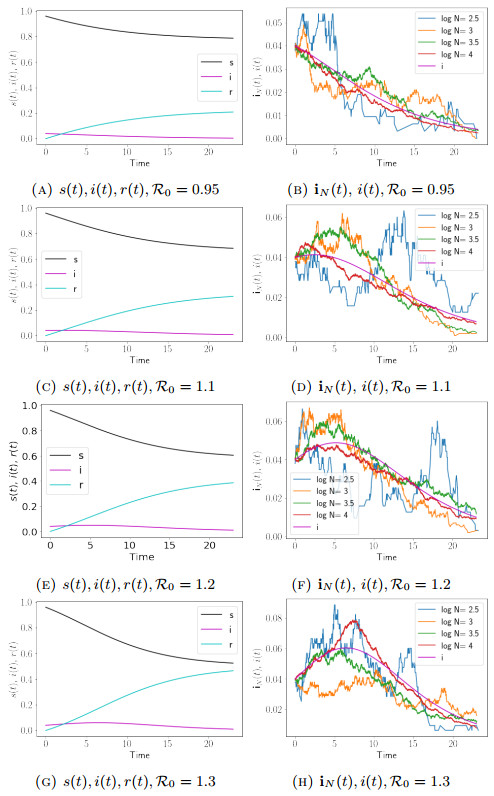
We focus on the cases when the reproduction number $\mathcal R _0$ is near the self-sustaining level of $\mathcal R _0 = 1$, as is typical in a scenario where public health measures trade off against economic and educational needs of the population¹. Specifically, we consider the cases when $\mathcal R _0 = 0.95$, $1.1$, $1.2,$ and $1.3$, respectively. Parameters of the simulations are recorded in figure caption.

¹As a specific example we note that the dynamic reproductive number has been estimated weekly in Los Angeles County using a Bayesian SEIR model applied to hospital demand data - during the period July 2020-April 2021 it remained within a 25% window of one [10].

In all the cases, we show output of the SIR-IPC model simulations with $N$ taking on values $10^{2.5}$, $10^{3}$, $10 ^{3.5}$, and $10^4$, by the blue, orange, green, and red lines, respectively, in Figs. 1b, 1d, 1f, 1h. For the case when $\mathcal{R}_0 = 0.95$, we infer from (25) that the parameters and data used to create the blue, orange, green, and red lines in Fig. 1b give rise to the same set of solution $(s(t), i(t), r(t))$ to the deterministic SIR Model. Therefore, we only display the deterministic output once in Fig. 1a. This same arrangement also applies to other cases with different values of $\mathcal R_0$, which are displayed in Figs. 1c, 1e, and 1g, respectively In all the figures, black, magenta, and cyan lines represent $s(t)$, $i(t)$, and $r(t)$ associated with the deterministic simulation, respectively.

The finite size effects are exhibited. As the population size decreases, deviations of dynamics of the stochastic SIR Model from its continuum equation increase. The same simulation output is also observed over other random paths.

4.   Mathematical analysis of the finite size effects

In Theorem 3.3, a global upper bound of the same order of magnitude of $1/N$ is derived and the result indicates the order of the magnitude of the martingale infinitesimal variances when $N \rightarrow \infty$. To further understand the martingale variances when N is relatively smaller, in this section, we analyze the finite size effects, based on the martingale formulation, and simulations are run which support our theoretical conclusion.

4.1.   Scaling property of the stochastic component

We analyze the deterministic and stochastic component of the martingale formulation with varying population size $N$. We fix the initial condition of the compartment fractions and denote them as

We analyze the martingale formulation of the stochastic SIR model with varying population size $N$. Applying (9) and (13) to $\left ( {\textbf{s}}_ { N} ( t), {\textbf{i}}_{ N} ( t), {\textbf{r}}_{ N} ( t) \right )$ over a small time step $\Delta t$, we obtain

By (13) and additivity of the variance in time for martingales, we have

where $\Delta\mathcal {M}_{ N }^{(l)} \left ( t \right ) = \mathcal {M}_{ N }^{(l)} \left ( t +\Delta t \right ) - \mathcal {M}_{ N }^{(l)} \left ( t \right )$, $l = 1, 2, 3$. This together with (27) implies that the infinitesimal variances are the key to estimate the infinitesimal standard deviation of the stochastic component, and the deviation of the trajectories of the evolution of the model from its deterministic component.

We perform estimates at the first time step. At time zero, from (14) - (16) we infer

which implies that the infinitesimal variances for the attractiveness are each inversely proportional to $N$:

This together with (28) implies that at the first time step we have

From (33) and (27) we infer that at the first time step a smaller value of ${N}$ leads to a larger deviation of the trajectory of $( {\textbf{s}}_{ N} ( \omega, t), {\textbf{i}}_{ N} ( \omega, t), {\textbf{r}}_{ N} ( \omega, t))$ from its deterministic component, and the hotspots develop temporal transience in the simulations. This explains the finite size effects at the first time step. This suggests that smaller value of ${N}$ leading to a larger deviation remains to be true at an arbitrary later time, namely,

which leads to a theory of the finite size effects at an arbitrary later time.

Next we estimate the right-hand-side of formulas (14) - (16), so that we can estimate $\mathcal {V}_{ N }^{(l)} \left ( t \right ), l = 1, 2, 3$, at later times for $t>0$. In the prior literature of stochastic partial differential equations (see e.g. [12,17,57,67,71]), usually Itô calculus is applied, as the infinitesimal variances are multiplied by Wiener processes, and the population or number of particles is required to be large, which does not fit with the cases on which our focus here.

We conjecture that formulas (29) - (31) can be written for an arbitrary $t>0$ with the same leading order:

If our conjecture above is true, then we can fix a time period $[T_1, T_2]$, and take average of both sides of (35) - (37) over the time period $[T_1, T_2]$, and obtain

where $\overline{\mathcal {V}_{ N }^{(l)} }$, $l = 1, 2, 3$ denotes the time average of the infinitesimal variance over this time period:

Here we slightly abuse the notation and omit the dependence of the time average over $T_1$ and $T_2$.

4.2.   Numerical simulations

To check the validity of (34), we perform direct simulations of the infinitesimal standard deviations, namely

Example output can be found in Figure. 2.

Figs. 2a, 2c, and 2e show results of $\sigma _{ N }^{(l)} \left ( t \right )$, $l = 1, 2, 3$, in the case with $\mathcal R_0 = 0.95 <1$. The blue, orange, green and red lines show results with the same realizations from simulations with the corresponding colors in Fig. 1b, respectively. Figs. 2b, 2d, and 2f show results of $\sigma _{N}^{(l)} \left ( t \right )$, $l = 1, 2, 3$, in the case with $\mathcal R_0 = 1.3 >1$. The blue, orange, green and red lines show results with the same realizations from simulations with the corresponding colors in Fig. 1h, respectively.

The output of the simulations supports the validity of (34). The same simulation results are also observed over other random paths.

We validate our conjecture of (38) - (40) through the following numerical simulation. Fig. 3 shows the log–log plot with error bars for (38) - (40). The lines show the theoretical scaling with slope as $-1$ and the $x$-intercepts as $\log ( p_1 \beta { {i}_0} { {s}_0})$, $\log ( p_1 \beta { {i}_0} { {s}_0} + p_2 \gamma { {i}_0})$, and $\log (p_2 \gamma { {i}_0} )$, respectively, and the error bars show the true scaling with the $x$-coordinate and $y$-coordinate as follows:

for $N = 10^{2.5},10^{3}, 10^{3.5}, 10^4$, and $l = 1, 2, 3.$ Here $[T_1, T_2]$ are chosen as $[0, 10]$, $[1, 11]$, $[2, 12]$, ..., and $[13, 23]$. The minimum and maximum values of $y = \log\left (\overline{\mathcal {V}_{ N }^{(l)}}\right)$, $l = 1, 2, 3$, taken over all such intervals are set as the limits of the error bars.

Figs. 3a, 3c, and 3e show results in the cases when $\mathcal{R}_0 = 0.95$ for $l = 1$, $2$, and $3$, respectively. The error bars with $x$-axis as $2.5$, $3$, $3.5$, and $4$ show results with the same realization from simulations of the blue, orange, green, and red lines in Fig. 1b, respectively. Figs. 3b, 3d, and 3f show results in the cases when $\mathcal{R}_0 = 0.13$ for $l = 1$, $2$, and $3$, respectively. The error bars with $x$-axis as $2.5$, $3$, $3.5$, and $4$, show results with the same realization from simulations of the blue, orange, green, and red lines in Fig. 1h, respectively.

The output shows that the error bars are short and fall mostly on the straight lines representing the theory. The same simulation results are also observed over other random paths. These results support the validity of equations (38) - (40) and our theory for the finite size effects based on the martingale formulation.

5.   Case studies of a small county and a cruise ship

In the following experiments, we set parameters to mimic real world cases of a small county or a cruise ship. And we will display plots for the fractional of compartment and the infinitesimal standard deviations, and analyze the role of stochastic variances in each case. The infinitesimal variances represent chance variations that leads to deviations from the deterministic SIR model. Through simulations of infinitesimal variances as in (14) - (16), we can produce envelopes that encompass a majority of the random paths. Realistically, our findings suggest that for small populations, the probabilities of rare events, e.g. the early-die-out or early-outbreak are important.

We study the outbreak of COVID-19 in Churchill County, Nevada from July, 2020 to March, 2021 and on the Diamond Princess cruise ship from February to March, 2020. Since early testing on the Diamond Princess was done by sampling from the population due to limited availability of testing, there is an under-reporting issue in the infected counts. The data of Churchill County was collected from [19] and the reported number of confirmed cases of Princess Diamond, and the quarantine process were retrieved from publicly available sources including the Princess Cruise website of the Carnival Cooperation [18] and the official website of Ministry of Health, Labor and Welfare, Japan (Ministry of Health, Labor and Welfare, Japan [54].

We plot the daily confirmed cases with 30 realisations from the SIR-IPC models in fig. 4. For fig. 4a, the total population is set to be Churchill County's population $N = 25715$ and the reproduction number $\mathcal R_0 = 1.007$ using linear regression optimized by a grid search. For fig. 4c the total population is set to be the total number of passengers and crew on Diamond Princess $N = 3711$. Cruise ships carry a large number of people in confined spaces with relative homogeneous mixing, amplifying an already highly transmissible disease. Following the estimation of the dynamic reproduction number in [60], we take an average of these estimates from Feb. 5 to Feb. 26, resulting in $\mathcal R_0 = 2.02$. With these smaller populations, the infinitesimal standard deviations are non-negligible in the stochastic SIR model. Public health officials thus need to be aware of the variability of possible outcomes due to finite size effects.

6.   Discussion

Compartmental models are a powerful tool to predict and control infectious diseases. In this article, we study theoretically and quantitatively the finite size effects arising in stochastic compartmental models, where individual realizations of the models deviate from their mean-field limit.

We apply compound Poisson processes to classical SIR compartmental models without vital dynamics. The result is a continuous-time Markov pure jump process, and a martingale approach can be applied to this process. The process is expressed as the sum of a deterministic and a stochastic component, which provides us with a tool to study both the statistical and stochastic features of the process. The deterministic part coincides with the classical deterministic SIR model. By providing a bound of the variances of the martingale, we show that the continuum mean-field limit is indeed the deterministic SIR model. Simulations results also align with the conclusion.

However, a small population size leads to stochastic fluctuations that deviate from the deterministic SIR model. Quantitative and theoretical analysis of these finite size effects have not been well-studied. We find a theoretical explanation for the finite size effects by observing that the stochastic component of the martingale formulation scales as the inverse of the square root of the population size. A larger variance both in the outbreak size and its temporal behavior arises as population size decreases. This scaling property is verified at time zero with equilibrium initial data. Direct numerical simulations of the theoretical infinitesimal variance support our theory as output shows that the dependence on population size remains to be true in later times. Here we simulate with fixed initial compartment fractions and vary the total population size. To the best of our knowledge, this is the first time that simulations of theoretical infinitesimal variances for stochastic compartmental models are implemented. In previous works only empirical variations are simulated (see e.g. [59], [33]), and the focus was on the effects of statistical fluctuations on the reproduction number assuming varying initial compartment fractions [4]. We also simulate finite size effects with small populations and analyze with real data. All the simulations support our theory. Our results exhibit the danger of fitting data collected during an outbreak to deterministic counterparts of the stochastic compartmental models, especially for small populations.

Finite size effects are observed in Markov processes for population dynamics in many fields ([15,26,28,29,32,36,41,42,55,65,66,70]). But there have been few quantitative studies to date about finite size effects in epidemics. On one hand, the methodology developed here may be broadly useful for quantitative social and natural sciences. On the other, this work provides a mathematical and theoretical framework that may contribute to epidemic policy for public health agencies.

So far, the analysis is purely theoretical. It remains an open problem to integrate the real-world data to the model and gleam some indicators from the data to control the disease. One example is that in order to control the spread, the government should know when and where to take certain measures to reduce $\beta$.

From Figure 5c, with a smaller population, the envelope of synthetic data can be wide. Additionally, the process with a smaller population also has more paths that die out early in the process(see fig. 2a, 2c, 2e), and 5a. Our work provides a good guide for authorities of smaller populations like cruise ships and small towns to estimate risk over time in order to prepare for the outbreak. It is important to bear in mind that the broader variations in the pandemic caused by the smaller population would lead to a wide outcome when it comes to estimating risk. In the past hundreds of years of human history, there have been several infectious diseases, including SARS, MERS and H1N1. However, only few of them, e.g. COVID-19 and 1918 influenza escalated into a pandemic. It is important to understand when, why and how a disease dies out and our next step is to quantitatively study the die-out event and its relations to finite size population and reproduction number $\mathcal{R}_0$.

Acknowledgments

We thank Professors Thomas Liggett, Jingyu Huang, Qiang Zeng, and Martina Hofmanova for helpful discussions.