


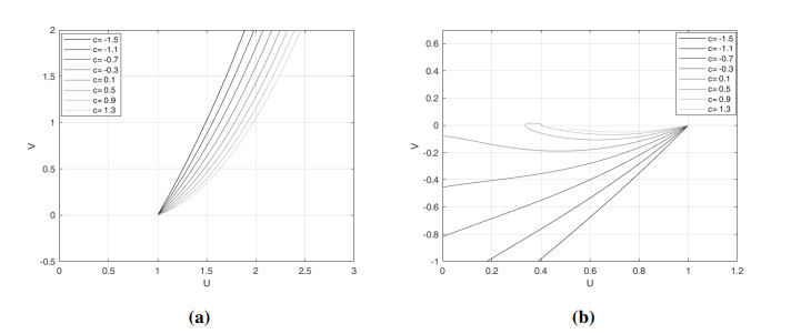
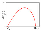
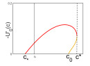
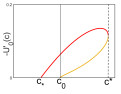
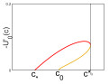
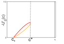
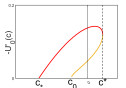
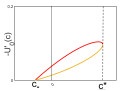
Figure 1.
Illustration of Lemma 3. As $ c $ increases, the unstable manifold of $ (1, 0) $ moves downward in the first quadrant (plot (a)), and upward in the fourth quadrant (plot (b)).
Citation: Rinaldo M. Colombo, Benedetto Piccoli. Preface[J]. Networks and Heterogeneous Media, 2011, 6(3): i-iii. doi: 10.3934/nhm.2011.6.3i
| [1] | José Luis Díaz Palencia, Abraham Otero . Modelling the interaction of invasive-invaded species based on the general Bramson dynamics and with a density dependant diffusion and advection. Mathematical Biosciences and Engineering, 2023, 20(7): 13200-13221. doi: 10.3934/mbe.2023589 |
| [2] | Wenhao Chen, Guo Lin, Shuxia Pan . Propagation dynamics in an SIRS model with general incidence functions. Mathematical Biosciences and Engineering, 2023, 20(4): 6751-6775. doi: 10.3934/mbe.2023291 |
| [3] | Tong Li, Zhi-An Wang . Traveling wave solutions of a singular Keller-Segel system with logistic source. Mathematical Biosciences and Engineering, 2022, 19(8): 8107-8131. doi: 10.3934/mbe.2022379 |
| [4] | Sung Woong Cho, Sunwoo Hwang, Hyung Ju Hwang . The monotone traveling wave solution of a bistable three-species competition system via unconstrained neural networks. Mathematical Biosciences and Engineering, 2023, 20(4): 7154-7170. doi: 10.3934/mbe.2023309 |
| [5] | Haiyan Wang, Shiliang Wu . Spatial dynamics for a model of epidermal wound healing. Mathematical Biosciences and Engineering, 2014, 11(5): 1215-1227. doi: 10.3934/mbe.2014.11.1215 |
| [6] | M. B. A. Mansour . Computation of traveling wave fronts for a nonlinear diffusion-advection model. Mathematical Biosciences and Engineering, 2009, 6(1): 83-91. doi: 10.3934/mbe.2009.6.83 |
| [7] | Li-Jun Du, Wan-Tong Li, Jia-Bing Wang . Invasion entire solutions in a time periodic Lotka-Volterra competition system with diffusion. Mathematical Biosciences and Engineering, 2017, 14(5&6): 1187-1213. doi: 10.3934/mbe.2017061 |
| [8] | Xiao-Min Huang, Xiang-ShengWang . Traveling waves of di usive disease models with time delay and degeneracy. Mathematical Biosciences and Engineering, 2019, 16(4): 2391-2410. doi: 10.3934/mbe.2019120 |
| [9] | Xixia Ma, Rongsong Liu, Liming Cai . Stability of traveling wave solutions for a nonlocal Lotka-Volterra model. Mathematical Biosciences and Engineering, 2024, 21(1): 444-473. doi: 10.3934/mbe.2024020 |
| [10] | Guo Lin, Shuxia Pan, Xiang-Ping Yan . Spreading speeds of epidemic models with nonlocal delays. Mathematical Biosciences and Engineering, 2019, 16(6): 7562-7588. doi: 10.3934/mbe.2019380 |
Models for the spread of invasive species have been studied for nearly a century now, starting with the work by Kolmogorov et al. [1] and Fisher [2]. For an excellent review, see [3]. Most of these models consider the landscape through which the species spreads as independent and unaffected by the presence of the species. However, many species, and, in particular, many invasive species, actively alter some physical attributes of the landscape through which they spread [4]. Those species are known as ecosystem engineers [5,6]; see also [7]. Usually, the engineering activity is beneficial to the species, but not always. Some species who can only survive after engineering are referred to as obligate engineers. Examples include burrowing fauna [8] and coastal redwoods [9]. Few models exist for the population dynamics of ecosystem engineers (see [9] and references therein), and only one that models their spread through a landscape explicitly [10]. Our work is closely related to [10], but we consider a strong Allee effect in the population dynamics.
An Allee effect is defined as a positive relationship between population density and per-capita growth rate [11]. It describes the effect that the presence of conspecifics can be beneficial for per-capita reproduction, at least at low enough densities. At high densities, per-capita reproduction usually decreases from competition with conspecifics. Typical mechanisms for an Allee effect are mate search and group defense [11]. A strong Allee effect occurs when the population is not viable below a certain threshold density. This is the case that we consider. In contrast, the authors in [10] considered a logistically growing population where there is no Allee effect. Typically, population dynamics models with Allee effect are much harder to study because they exhibit bistability so that the linearization at the zero state does not give information about the existence and stability of a positive state. In the context of mathematical models for species spread, explicit formulas for the speed of spread are often available when there is no Allee effect [3] but practically never when there is an Allee effect, the exception being the work by Hadeler and Rothe [12], which we will use and expand here.
The standard modeling framework for biological invasions are reaction–diffusion equations that track the density $ u = u(t, x) $ of the invading species in space $ x $ and time $ t $ [3]. In one spatial dimension, they read
|
$ ut=Duxx+f(u),x∈(−∞,∞),t>0, $
|
(1.1) |
where $ D $ is the diffusion coefficient and $ f = f(u) $ the population growth term, which may or may not include an Allee effect. Traveling waves are special solutions of this equation of the form $ u(t, x) = U(x-ct) $, where $ U $ is the wave profile and $ c $ the wave speed. As asymptotic boundary conditions, $ U $ connects two steady states, i.e., two zeros of $ f $. For example, in the original Fisher equation with logistic growth function $ f(u) = u(1-u) $, monotone traveling waves connecting the state 1 to the state 0 exist for all speeds $ c\geq 2\sqrt{Df'(0)} $ [2]. In contrast, with the Allee growth function $ f(u) = u(1-u)(u-a) $, a monotone traveling wave connecting those two states exists only for the speed $ \sqrt{2} D(0.5-a) $ [12]. In particular, while traveling waves with a logistic growth function always have positive speed, i.e., the species invades empty habitat, traveling waves with Allee growth function can have negative speeds, i.e., the species retreats.
Many generalizations of (1.1) exist. The two most relevant to our work are the extensions to free boundary problems by Du and Lin [13] and by Lutscher et al. [10]. In the first case, the authors divide the landscape into a bounded invaded part (where the population is present) and its unbounded non-invaded complement (where it is not). They model the population density on the (bounded) invaded portion by a reaction-diffusion equation as above and the movement of the boundary between the invaded and non-invaded parts of the landscape by a Stefan-like condition [13]. This condition was originally derived for the melting of ice on the surface of a lake and relates the speed of the boundary to the gradient in the density via heat transfer considerations [14]; see also [15]. The boundary condition has been rederived from ecological considerations in [16]. The existence of solutions and spreading properties in higher dimensions were investigated in the radially symmetric [17] and the general case [18]. Later, the work was extended to competing species [19] and to moving habitats [20]. Several different interface conditions, including nonlocal ones, were derived and the corresponding propagation behavior analyzed, for example conditions that resulted from delays [21], from density-dependent diffusion without and with Allee effect [22,23], and from considering a perception range of individuals [24]. Other authors have considered retreating boundaries [25]. For a recent review of these developments, see also the references in [26].
In contrast, the approach in [10] divides the landscape into an engineered (where population growth is possible) and non-engineered part (where it is not). They model the population density in each part by a reaction–diffusion equation as in (1.1), but the growth function in the non-engineered part is negative, indicating population decline. The matching conditions of population density and flux between the engineered and non-engineered parts were derived in a slightly different context from random walks in [27]. From the same mechanistic basis, the authors in [10] derived conditions for the movement of the boundary between the engineered and non-engineered parts based on three scenarios of how the engineering process takes place (see next section). They then study the existence of traveling waves when there is no Allee effect; here we study traveling waves with strong Allee effect.
In the next section, we present the model and define all the necessary terms. The model is a two-sided free boundary problem with nonstandard matching conditions at the boundary. Then, we split the analysis in two parts. In Section 3, we consider traveling waves with a given speed. We call these forced waves. They do not (necessarily) satisfy the equation for the speed of the free boundary, but they are an important intermediate step to study the existence of traveling waves to the free boundary problem. They arise as equations in their own right when studying externally forced systems, such as moving-habitat models, where the forcing corresponds to the optimal temperature zones for a species moving due to climate change [28]. We show that there is a great variety of qualitatively different wave forms, much larger than in [10], where the growth function did not have an Allee effect, and much larger than in [12], where the landscape was homogeneous. In Section 4, we use the results from the preceding section to study traveling waves of the free boundary problem; we refer to these as free traveling waves. Most of our methods involve geometric considerations of phase-plane equations for the traveling waves. We summarize our results in various tables since there are many cases to consider. We present most but not all of the proofs here; we omit those that follow by the same ideas as for other proofs. More details can be found in [29].
Our model here is essentially the same as the model in [10], but with a bistable growth function instead of the monostable growth function used there. Hence, we keep the model description brief and refer to [10] for details. We let $ u(t, x) $ denote the density of the species at time $ t > 0 $ in location $ x\in \mathbb{R} $. We have two habitat types: engineered and non-engineered. The engineered habitat is suitable for population growth, but the non-engineered habitat is not. The engineering activity moves the boundary between these two types of habitat. We denote by $ x = L(t) $ the location of the interface between engineered and non-engineered habitat at time $ t $, and choose the region $ (-\infty, L(t)) $ as the engineered habitat and $ (L(t), +\infty) $ as the non-engineered habitat.
Movement and demographics in the engineered habitat are modeled by
|
$ ut=D1uxx+f(u),(t,x)∈(0,∞)×(−∞,L(t)), $
|
(2.1) |
where $ D_1 > 0 $ is the diffusion coefficient and $ f $ is the (net) growth function
|
$ f(u)=r(u−k0k1)(1−uk1)u $
|
(2.2) |
with rate $ r > 0 $, carrying capacity $ k_1 > 0 $, and Allee threshold $ 0\leq k_0 < k_1 $. Movement and mortality in the non-engineered habitat are modeled by
|
$ ut=D2uxx−mu,(t,x)∈(0,∞)×(L(t),∞), $
|
(2.3) |
where $ D_2 > 0 $ is the diffusion coefficient and $ m > 0 $ is the death rate.
At the interface between the two habitat types, an individual moves to the engineered habitat with probability $ \alpha_1 $, to the non-engineered habitat with probability $ \alpha_2 $, and stays at the boundary with remaining probability $ \alpha = 1-(\alpha_1+\alpha_2) $. The resulting matching condition for the density at the interface is
|
$ α2D1u(t,L(t)−)=α1D2u(t,L(t)+), $
|
(2.4) |
where superscripts $ \pm $ denote one-sided limits [27]. The matching conditions for the population fluxes at the interface reflect the fact that the movement process at the interface conserves the total population. As in [28], conservation of mass leads to
|
$ D1ux(t,L(t)−)+L′(t)u(t,L(t)−)=D2ux(t,L(t)+)+L′(t)u(t,L(t)+). $
|
(2.5) |
We have three different scenarios for the movement of the interface due to the engineering activity; please see [10] for the detailed derivations.
Scenario 1: Individuals at the interface transform the neighboring non-engineered habitat and thereby move the boundary. The movement of the boundary is proportional to the density of the species at the boundary, i.e.,
|
$ L′(t)=2D1ηαu(t,L(t)−), $
|
(2.6) |
where $ \eta $ is a proportionality constant. If $ \alpha = 1-(\alpha_1+\alpha_2) > 0 $, then $ L'(t) > 0 $ and the boundary is expanding. If $ \alpha = 0 $, i.e., no individual stays at the boundary, then $ L'(t) = 0 $ and the boundary does not move.
Scenario 2: If the engineered structure requires maintenance, a certain population density is required for the boundary to expand; otherwise it will retract. The expression is
|
$ L′(t)=2D1ηα(u(t,L(t)−)−ˉu), $
|
(2.7) |
where $ \bar{u} $ is the threshold density, and $ D_1 $ and $ \eta $ are as in Scenario 1.
Scenario 3: If individuals leave the engineered habitat and move the boundary due to pressure from higher density behind them, one arrives at the Stefan-type condition
|
$ L′(t)=−2ηD1ux(t,L(t)−). $
|
(2.8) |
The three scenarios can be combined in a single equation as
|
$ L′(t)=B(u,ux)|(t,L(t)−), $
|
(2.9) |
where $ B $ can be one of the expressions (2.6), (2.7), or (2.8). Note that only scenario 2 allows $ L'(t) < 0 $.
After nondimensionalization, our system becomes
|
$ {ut=uxx+u(u−a)(1−u),x<L(t),t>0,ut=Duxx−˜mu,x>L(t),t>0,α2u(t,L(t)−)=α1Du(t,L(t)+),t>0,(ux+L′(t)u)|(t,L(t)−)=(Dux+L′(t)u)|(t,L(t)+),t>0,L′(t)=˜B(u,ux),t>0. $
|
(2.10) |
where $ \widetilde{B} $ is the scaled version of (2.6), (2.7), or (2.8), that is,
|
$ L′(t)=η1αu(t,L(t)−), $
|
(2.11) |
|
$ L′(t)=η1α(u(t,L(t)−)−ˉu), $
|
(2.12) |
|
$ L′(t)=−η2ux(t,L(t)−). $
|
(2.13) |
The nondimensional parameters are
|
$ D:=D2D1,a:=k0k1,˜m=mr,η1:=2k1η√D1r,η2:=2ηk1. $
|
(2.14) |
We drop the tilde to simplify notation. All parameters are nonnegative and $ 0 < a < 1 $ as well as $ 0 < \alpha_1+\alpha_2 < 1 $. Since movement in favorable habitat is typically slower than in unfavorable habitat [30], we can assume that $ D_1\leq D_2 $. Since individuals typically prefer engineered over non-engineered habitat, we can also assume that $ \alpha_1\geq \alpha_2 $. Therefore, we assume that
|
$ Δ:=α2D1α1D2=α2α1D<1. $
|
(2.15) |
We studied the existence of solutions to the above system in [31]. Here, we consider solutions in the form of traveling waves, i.e.,
|
$ u(t,x)=U(x−ct)=U(z),L(t)=l0+ct, $
|
(2.16) |
with asymptotic conditions $ U(-\infty) = 1 $ and $ U(\infty) = 0 $. Without loss of generality, we may assume that $ l_0 = 0 $. Therefore, a traveling wave solution of our model satisfies
|
$
\begin{array}{*{20}{c}}
{\left\{ {\begin{array}{*{20}{l}}
{ - cU' = U'' + f(U), }&{\;z < 0, }\\
{ - cU' = DU'' - mU, }&{\;z > 0, }\\
{U'({0^ - }) + cU({0^ - }) = DU'({0^ + }) + cU({0^ + }), }&{}\\
{{\alpha _2}U({0^ - }) = {\alpha _1}DU({0^ + }), }&{}\\
{U( - \infty ) = 1, }&{}\\
{U(\infty ) = 0, }&{}\\
{c = \widetilde B(U({0^ - }), U'({0^ - })), }&{}
\end{array}} \right.}&\begin{array}{l}
(2.17)\\
(2.18)\\
(2.19)\\
(2.20)\\
(2.21)\\
(2.22)\\
(2.23)
\end{array}
\end{array}
$
|
where $ f(U) = U(U-a)(1-U) $, and $ \widetilde{B} $ is one of the expressions (2.11), (2.12) or (2.13).
We study the existence of traveling waves in two steps. First, we consider speed $ c $ as a parameter and determine the range of $ c $ for which the reduced model (2.17)–(2.22) has traveling waves. We refer to these as forced traveling waves. Then, we consider the feedback from the dynamics to the speed via the moving boundary condition. We determine when and under what conditions the speed can be in the range that we obtained in the first step. We refer to the resulting solutions as free traveling waves.
The reduced model (2.17)–(2.22), with speed $ c $ as a parameter, is an interesting system to study in its own right. It generalizes the model by Hadeler and Rothe for traveling waves in a reaction–diffusion equation with Allee effect on the entire real line; see Section 6 in [12]. In fact, we shall use their results below. In their model, the habitat is homogeneous, whereas in our model, it consists of the two types with correspondingly different movement and demography. As the interface between the two habitat types shifts at speed $ c $, our model becomes one of forced waves [32]. Such forced waves emerge from the study of so-called moving-habitat models that describe the geographic shift in optimal temperature conditions due to climate change [33]. There are two kinds of moving habitat models: those with one interface [34] that separates the favorable from the unfavorable habitat, and those with two [28]; see [35] for a recent review. A typical result for a single-interface model is that if the unfavorable habitat expands too quickly, then the species in the shrinking favorable habitat cannot persist. These models have been studied without Allee effect [34] and with weak Allee effect [36]. In contrast, in our model the favorable habitat can expand with the activity of the ecosystem engineer, and we consider a strong Allee effect. For the two-interface model, the existence of traveling pulses under certain conditions has been shown without [37] and with [38] Allee effect.
We formulate the forced-wave problem (2.17)–(2.22) with parameter $ c $ as an equivalent phase-plane problem. The proof of the following lemma is essentially the same as in [10].
Lemma 1. Solutions of (2.17)–(2.22) with speed $ c $ are equivalent to solutions of
|
$ U′=V,V′=−f(U)−cV, $
|
(3.1) |
where $ f(U) = U(U-1)(1-U), $ with
|
$ U(−∞)=1,V(−∞)=0, $
|
(3.2) |
and
|
$ V(0)=bU(0), $
|
(3.3) |
where
|
$ b=Δ(c2−√c24+Dm)−candΔ=α2α1D. $
|
(3.4) |
The steady states of the phase-plane equations (3.1) are $ (0, 0), $ $ (1, 0) $, and $ (a, 0) $. Hence, by (3.2) and (3.3), our forced traveling waves are solutions in the phase plane that connect the steady state $ (1, 0) $ with the straight line $ V = bU $. In other words, we are looking for intersections of an unstable manifold of $ (1, 0) $ with the line $ V = bU $. We call such a connection a traveling wave orbit (TWO).
Hadeler and Rothe [12] studied traveling waves on the whole real line; hence, their boundary conditions were given at $ \pm\infty $. They found two critical values of speed, $ c_0 $ and $ c_m $. At $ c = c_0 $, a unique monotone traveling wave exists, connecting $ 1 $ with $ 0 $. This solution corresponds to a heteroclinic orbit of (3.1), connecting $ (0, 0) $ and $ (1, 0) $. In addition, $ c = c_m $ is the minimal speed for the existence of a monotone decreasing traveling connecting $ 1 $ to $ a $. This solution corresponds to a heteroclinic orbit of (3.1), connecting $ (1, 0) $ and $ (a, 0) $. The explicit formulas for these critical values are
|
$ c0:=√2(12−a),c1:=2√f′(a)=2√a(1−a),c2:=(1+a)√2,cm:={c2,for0<a≤13,c1,for13<a<1. $
|
(3.5) |
To find the required TWO in our system, we study the properties of the function $ b(\cdot) $ that defines the boundary condition of (3.3) and the qualitative behavior of the steady states.
Lemma 2. For $ 0 < \Delta < 1 $, the expression $ b = b(c) $ in (3.4) has the following properties:
i) $ \lim_{c\to \infty}b(c) = -\infty $.
ii) $ b $ is monotone decreasing in $ c $.
iii) $ b $ changes sign at
|
$ c∗:=−√Δ21−ΔD2m<0. $
|
(3.6) |
Proof. Parts $ i) $ and part $ ii) $ follow directly from the definition in (3.4). To prove part $ iii) $, we set $ b(c) = 0 $ and simplify to find $ c^2(1-\Delta) = \Delta^2D_2m. $ For $ 0 < \Delta < 1 $, this equation has real roots, among which the negative one is $ c_* $. For $ c > c_* $, we have $ b < 0 $.
The eigenvalues of the Jacobian at the steady states of (3.1) are given by
|
$ λ±i(c)=12(−c±√c2−4f′(i)),for i=0,a,1. $
|
(3.7) |
The steady states $ (0, 0) $ and $ (1, 0) $ are saddle points. Depending on the value of $ c $, $ (a, 0) $ can be an unstable node ($ c\leq -2 \sqrt{f'(a)} $), an unstable focus ($ -2 \sqrt{f'(a)} < c < 0 $), a center ($ c = 0 $), a stable focus ($ 0 < c < 2 \sqrt{f'(a)} $), or a stable node ($ c\geq2\sqrt{f'(a)} $).
We denote the unstable manifold of the point $ (1, 0) $ by $ M = M(c) $ and study how it depends on parameter $ c $. The manifold consists of two parts: one that leaves $ (1, 0) $ into the first quadrant and one that leaves into the fourth quadrant. The latter connects with the stable manifold of $ (0, 0) $ to form a heteroclinic connection if, an only if, $ c = c_0 $ (see above). When $ c < c_0 $, it leaves the fourth quadrant into the third quadrant; when $ c > c_0 $, it leaves into the first quadrant. If it leaves into the first quadrant, it may return into the fourth quadrant and oscillate around $ (a, 0) $ if that point is a spiral.
Lemma 3. The unstable manifold of $ (1, 0) $, $ M(c) $, changes monotonically with respect to $ c $ in the following sense:
i) The part of $ M(c) $ leaving $ (1, 0) $ into the first quadrant moves downward as $ c $ increases: $ M(c') $ lies above $ M(c'') $ in the first quadrant if $ c' < c'' $.
ii) The part of $ M(c) $ in the fourth quadrant between $ (1, 0) $ and its first intersection with the positive part of $ U $-axis or negative part of $ V $-axis moves upward as $ c $ increases: $ M(c'') $ lies above $ M(c') $ in the fourth quadrant if $ c' < c'' $, at least until the first intersection with the axes.
Proof. The unstable manifold $ M $ of $ (1, 0) $ is tangent to the line $ V = \lambda^+_1(U-1) $ at $ (1, 0) $. From the expression in (3.7), we see that $ \frac{d\lambda^+_1}{dc} < 0 $. Hence, for $ c' < c'' $, $ M(c'') $ lies below $ M(c') $ in the first quadrant near $ (1, 0) $. We show that there is no intersection between $ M(c') $ and $ M(c'') $ in the first quadrant. To the contrary, assume $ (\bar{U}, \bar{V}) $ is the point with the smallest value of $ \bar{U} > 1 $ and $ \bar{V} > 0 $, where the two unstable manifolds $ M(c') $ and $ M(c'') $ intersect. The slope of the vector field at that point is
|
$ dVdU=V′U′=−f(ˉU)−cˉVˉV=−f(ˉU)ˉV−c. $
|
(3.8) |
Since $ c' < c'' $, the slope of $ M(c') $ is steeper than that of $ M(c'') $ at the intersection point. However, this implies that for $ U < \bar{U} $, $ M(c'') $ lies above $ M(c') $. This contradicts the above observation based on the linearization near $ (1, 0) $. Hence, there is no such intersection. Similar reasoning can be applied in the fourth quadrant to prove part $ ii) $. The statement of the lemma is illustrated in Figure 1.
Hadeler and Rothe describe seven different types of traveling fronts in their system, some monotone, some oscillating, but only one that connects 1 to zero; see Theorem 13 in [12]. We are only interested in those forced waves that connect 1 with zero, but we find the following four qualitatively different types in our system.
Definition 1. i) If the TWO is entirely in the fourth quadrant, we say that the wave is of type Ⅰ (TW-Ⅰ).
ii) If the TWO begins and ends in the fourth quadrant but crosses into the first quadrant in between, we say that the wave is of type Ⅱ (TW-Ⅱ).
iii) If the TWO begins in the fourth quadrant and ends in the first, we say that the wave is of type Ⅲ (TW-Ⅲ).
iv) If the TWO is entirely in the first quadrant, we say that the wave is of type Ⅳ (TW-Ⅳ).
We illustrate the different possible qualitative shapes of TW-Ⅰ in Figure 2 and the three other types in Figure 3. Clearly, TW-Ⅰ and TW-Ⅱ require the slope of the boundary line $ V = bU $ to be nonpositive, i.e., $ c\leq c_* $ (see (3.6)), while TW-Ⅲ and TW-Ⅳ require $ b $ to be positive, i.e., $ c > c_* $. At $ c = c_* $, the slope of the boundary line is zero so that the intersection of the unstable manifold $ M $ and the boundary line occurs on the $ U $-axis. This can happen in two ways. If $ c_* < c_0 $, then $ M(c_*) $ lies below $ M(c_0) $ (Lemma 3), which is the heteroclinic orbit between $ (1, 0) $ and $ (0, 0) $. In particular, $ M(c_*) $ does not intersect the $ U $-axis, except at $ (1, 0) $; see Figure 2(e). If $ c_* > c_0 $, then there are two intersections of $ M(c_*) $ and the $ U $-axis, one at $ (1, 0) $ and one at $ (U_*, 0) $ for some $ 0 < U_* < a $; see Figure 2(g). When the intersection occurs at $ (1, 0) $, the resulting traveling wave is equal to the constant $ U = 1 $ for $ z < 0 $; see Figure 2(f). At $ c_* = c_0 $, there is a heteroclinic orbit connecting $ (1, 0) $ with $ (0, 0) $ so that the only admissible intersection of $ M $ and the $ U $-axis is at $ (1, 0) $.


More than one traveling wave of the same type (except for TW-Ⅳ) may exist for a given speed. It is also possible that we have traveling waves of different types for the same speed; see Figure 4.

Looking at the different TWOs in Figures 2 and 3, it is clear that in addition to the speed parameter ($ c $), the Allee threshold parameter ($ a $) plays a crucial role in determining which TWOs are possible because the two together determine the behavior near $ (a, 0) $. Hence, we organize our results on the existence of traveling waves according to these two parameters. Following [12], we divide the $ a $–$ c $ plane based on the behavior of the part of the unstable manifold $ M = M(c) $ that enters the fourth quadrant; see Figure 5.

In region 1 (blue), $ M $ leaves the fourth quadrant through the negative vertical axis. Hence, according to Definition 1, only TW-Ⅰ may appear here. In region 2 (red), $ M $ is a heteroclinic connection from the saddle at $ (1, 0) $ to the stable focus at $ (a, 0) $. TW-Ⅰ and TW-Ⅱ may exist here. In region 3 (gray), $ M $ leaves the fourth quadrant through the horizontal axis and approaches the part of $ M $ that enters the first quadrant. Only TW-Ⅰ and TW-Ⅲ may appear here. In regions 0 (green) and 4 (yellow), $ M $ is a heteroclinic connection from the saddle at $ (1, 0) $ to the stable node at $ (a, 0) $. Only TW-Ⅰ may exist in these regions, but we will show below that no TW-Ⅰ can exist in region 0. All of these regions only indicate where certain waves are possible. To show when they actually occur, we determine certain threshold values of the speed and then discuss each wave type separately. We begin with an upper limit for the existence of waves.
Theorem 1. There exists a threshold value of speed above which there is no traveling wave of any type; for any speed below the threshold, there exists at least one traveling wave of some type.
Proof. We need to show that for all speeds $ c $ above some threshold, there is no intersection between the boundary line, $ V = b(c)U $, and the unstable manifold, $ M(c) $. For $ c = c_0 $, we have a heteroclinic connection between $ (1, 0) $ and $ (0, 0) $. The slope of the heteroclinic at $ (0, 0) $ is given by the eigenvalue $ \lambda_0^-(c_0) $; see (3.7). The boundary line at this speed, $ V = b(c_0)U $, may be above or below this connection. Accordingly, we divide our proof into the following cases.
Case 1: $ b(c_0)\leq \lambda_0^-(c_0) $, i.e., the boundary line is below the tangent line to the heteroclinic when $ c = c_0 $. In this case, the boundary line and the heteroclinic intersect only at $ (0, 0) $. Necessarily, we have $ c_* < c_0 $ as $ b(c_0) < 0 $. By Lemmas 2 and 3, we know that as $ c $ increases, $ M(c) $ and $ V = b(c)U $ move in opposite directions in the fourth quadrant. Hence, they will not intersect for $ c > c_0 $. However, as in Lemma 3.6 in [10], the part of $ M(c) $ that enters the fourth quadrant will exit it through the negative $ V $-axis for all $ c < c_0 $. Hence, it must intersect the boundary line as long as $ c > c_* $. Hence, we have a TW-Ⅰ for $ c_*\leq c < c_0 $. On the other hand, as the slope of the boundary line becomes positive for $ c < c_* $, the boundary line will intersect the part of $ M(c) $ that enters the first quadrant so that a TW-Ⅳ appears; see also Theorem 5. Therefore, our threshold value here is $ c_0 $.
Case 2: $ b(c_0) > \lambda_0^-(c_0) $, i.e., the boundary line is above the tangent line to the heteroclinic when $ c = c_0 $. In this case, it may be possible to have $ c_0\leq c_* $ as $ b(c_0) $ may be positive. Hence, we divide our proof for this case into the following sub-cases:
Case 2.1: $ c_* < c_0 $. Similar to Case 1, we can show that at least one of TW-Ⅰ or TW-Ⅳ exists for $ c\leq c_0 $. Next, we choose $ \bar{c} > c_0 $ such that $ b(\bar{c}) < \lambda_0^-(c_0) $. The unstable manifold $ M(\bar{c}) $ lies above the heteroclinic connection, and exits the fourth quadrant through the $ U $-axis between $ 0 $ and $ a $. Therefore, there is no intersection between the boundary line $ V = b(\bar{c}) U $ and $ M(\bar{c}) $. Hence, by continuity of the phase plane with respect to $ c $, there is a maximal speed above which there is no traveling wave solution. For speeds less than this maximal speed and greater than $ c_0 $, we may have TW-Ⅱ in addition to TW-Ⅰ.
Case 2.2: $ c_*\geq c_0 $. For all $ c > c_0 $, we have $ b(c) < b(c_0) $, so that the part of $ M(c) $ that enters the fourth quadrant exits to the first quadrant. Therefore, we obtain the existence of a maximal speed as in Case 2.1. For speeds between $ c_* $ and the maximal speed, we obtain TW-Ⅰ and may have TW–Ⅱ as well. For $ c_0 < c < c_* $, we have TW-Ⅲ and TW-Ⅳ. Finally, for $ c\leq c_0 $, we only have TW-Ⅳ; see Figure 5 for illustration.
We can characterize the threshold speed as the speed for which the unstable manifold at $ (1, 0) $ is tangent to the boundary line; see Figure 6. As $ c $ increases, the boundary line moves downward whereas the portion of the unstable manifold between $ (1, 0) $ and its first intersection with the $ U $ axis moves upward. Hence, they cannot intersect for any larger speed. We call this maximal speed $ c^* $. We may or may not have a TWO for $ c^* $, as the following consideration shows.

Corollary 1. i) If
|
$ Dm≥2aΔ(aΔ+(12−a)), $
|
(3.9) |
then $ c^* = c_0 $ is the supremum of speeds for which a TWO exists.
ii) If (3.9) does not hold, then $ c^* $ is the maximum of speeds for which a TWO exists.
Proof. Inequality (3.8) is equivalent to $ b(c_0)\leq \lambda_0^-(c_0) = -\sqrt{2}/2 $. As seen in the proof of Theorem 1, in this case, the threshold value for the existence of a traveling wave is $ c^* = c_0 $. However, as the boundary line $ V = b(c_0)U $ only intersects $ M(c_0) $ at $ (0, 0) $, there exists no TWO at $ c = c_0 $. If (3.9) does not hold, our threshold value satisfies $ c^* > c_0 $. Hence, the tangency point has a positive $ U $-coordinate and the TWO connecting $ (1, 0) $ and the boundary line corresponds to a TW-Ⅰ at $ c^* $.
Unfortunately, there is no explicit formula for $ c^* $ when $ c^* > c_0 $, but it can be bounded by $ c_m $ as defined in (3.5).
Lemma 4. We have $ c_0\leq c^* < c_m $.
Proof. When $ c < c_0 $, we have either a TW-Ⅰ or TW-Ⅳ (see proof of Theorem 1). Hence, the lower bound is clear. By part $ i) $ of Theorem 13 in [12], there exists a heteroclinic connection between the steady states $ (1, 0) $ and $ (a, 0) $ for $ c\geq c_m $. This heteroclinic connection is tangent to $ V = \lambda_a^+(c)(U-a) $ at $ (a, 0) $ [39]. If we compare the slope of the boundary line and this tangent line, we see
|
$ b(c)=−c−Δ2(√c2+4Dm−c)<−c<12(−c+√c2−4a(1−a))=λ+a(c), $
|
for all $ c\geq c_m $. This implies that there cannot be any intersection between the boundary line and the heteroclinic connection for $ c\geq c_m $. Hence, we must have $ c^* < c_m $.
We now consider the effect of parameter $ a $. For $ 0 < a\leq1/2 $, we have $ c_0\geq0 $. By Lemma 4, we know that $ c^*\geq c_0 $. Therefore, in this case, we always have $ c^*\geq 0 $. However, for $ a > 1/2 $, the situation is not as straightforward because there is a homoclinic connection of $ (1, 0) $ that contains $ (a, 0) $ in its interior when $ c = 0 $.
Lemma 5. Let $ 1/2 < a < 1 $. If the boundary line $ V = b(0)U $ lies below the homoclinic connection of $ (1, 0) $ at $ c = 0 $ (resp., is tangent to it), then $ c^* < 0 $ (resp., $ c^* = 0 $). Otherwise, $ c^* > 0 $.
Proof. As seen in Lemmas 2 and 3, as $ c $ increases, the boundary line $ V = b(c)U $ and the unstable manifold $ M(c) $ move in different directions. Hence, knowing the location of the boundary line and the unstable manifold, which is part of the homoclinic connection at $ c = 0 $, will determine the sign of $ c^* $. If at $ c = 0 $ the boundary line is tangent to the homoclinic connection, then, as $ c $ increases, the boundary line moves downward and the part of $ M(c) $ in the fourth quadrant moves upward. Therefore, there will be no intersection for $ c > 0 $, and so $ c^* = 0 $. Similarly, if the boundary line lies below the homoclinic connection at $ c = 0 $, then there is no intersection for $ c\geq0 $. Therefore, the tangency condition for $ c^* $ must happen for some negative value of $ c. $ It turns out that one can find the parameter relation for which $ c^* = 0 $, however, the expressions are long; details can be found in Lemma 3.3.10 in [29]
Remark 1. We defined the maximal speed $ c^* $ such that for $ c > c^* $, there exists no traveling wave solution of any type. In fact, we shall see that $ c^* $ is the maximal speed for TW-I, while other types have different maximal speeds. Using similar arguments to those above, one can show that the maximal speed for TW-II, $ c^{**} $, say, satisfies $ 0 < c^{**} < c^* $. We will prove below that the maximal speed for TW-III and TW-IV is $ c_* $.
Theorem 2. For $ 0 < a < 1 $ and $ c_*\leq c < c^* $, there exists at least one forced wave of type I in (3.1)–(3.3). When $ c^* > c_0 $, we have a TW-I at $ c = c^* $ as well. When $ c_0 > c_* $, the TW-I is unique for $ c_*\leq c\leq c_0 $.
Proof. The proof of existence is similar to the proofs of Theorem 1 and Corollary 1. It remains to prove uniqueness for $ c_*\leq c\leq c_0 $, when $ c_0 > c_* $. We assume that there is more than one intersection between the boundary line $ V = b(c)U $ and the unstable manifold $ M(c) $ in the fourth quadrant for $ c_* < c < c_0 $. Then, at one of these intersections, the slope of the unstable manifold must be less than that of the boundary line (negative and steeper). We show that such an intersection point does not exist in the fourth quadrant when $ c_* < c < c_0 $. We split the proof into two cases according to whether the boundary line $ V = b(c)U $ is above or below the the tangent line to the heteroclinic connection at $ (0, 0) $.
Case 1: $ b(c) > \lambda_0^-(c_0) $. In this case, for $ c < c_0 $, there exists only one intersection between the boundary line $ V = b(c)U $ and the heteroclinic connection of $ (1, 0) $ and $ (0, 0) $ at some point $ (\bar{U}, \bar{V}) $ with $ \bar{U} > 0 $. There cannot be any intersection between the boundary line and the unstable manifold $ M(c) $ for $ 0 < U < \bar{U} $ because the boundary line is above the heteroclinic connection, while the unstable manifold is below it for $ c < c_0 $.
On the other hand, by its definition in (3.4), we have $ b(c) < -c $ for all $ c $. At $ U = a $, we have $ f(U) = 0 $, and, hence, $ dV/dU = -c $. So, at any point $ (U, V) $ in the fourth quadrant with $ a < U < 1 $, we have
|
$ dVdU=−c+f(U)−V=−c+f(U)|V|>−c>b(c). $
|
(3.10) |
as $ f(U) > 0 $ for $ a < U < 1 $. Hence, for $ a < U < 1 $, the slope of the unstable manifold is greater than that of the boundary line.
When $ \bar{U} > a $, the slope of the vector field, and, hence, the slope of the unstable manifold, is bigger than the slope of the boundary line for all points $ (U, V) $ with $ a < \bar{U} < U < 1 $ and $ V < 0 $, due to the above argument.
When $ \bar{U} < a $, we need to check the slope of the vector field where $ \bar{U} < U < a $. When $ 0 < U < a $, the heteroclinic is decreasing and concave up and $ f(U) < 0 $. In addition, for $ V_2 < V_1 < 0 $ and for fixed $ 0 < U < a $, we have
|
$ −c−f(U)V2=−c+|f(U)|V2>−c+|f(U)|V1=−c−f(U)V1. $
|
(3.11) |
Hence, for fixed $ U $, if we decrease $ V < 0 $, the slope of the vector field increases. Now we study the vector field in the region with $ \bar{U} < U < a $. At $ (\bar{U}, \bar{V}) $, we have
|
$ dVdU|(ˉU,ˉV)>b(c). $
|
(3.12) |
At any point $ (U_1, V_1) $ on the heteroclinic connection with $ \bar{U} < U_1 < a $ and $ V_1 < \bar{V} $, we have
|
$ dVdU|(U1,V1)>b(c), $
|
(3.13) |
because the heteroclinic connection is concave up. At any point $ (U_1, V_2) $ on the boundary line with $ V_2 < V_1 < \bar{V} $, we have
|
$ dVdU|(U1,V2)>b(c), $
|
(3.14) |
because of (3.11). Hence, for $ \bar{U} < U < a $, the slope of the vector field is bigger than the slope of the boundary line for $ c_* < c < c_0 $.
In summary, independent of $ \bar{U} $, the slope of the unstable manifold $ M(c) $ is greater than the slope of the boundary line $ V = b(c)U $ at all points $ (U, V) $ with $ \bar{U} < U $ and $ V < 0 $. So, there cannot be any intersection point at which the slope of the manifold is smaller than the slope of the boundary line. Therefore, the intersection between the boundary line $ V = b(c)U $ and the unstable manifold $ M(c) $ is unique for $ c_* < c < c_0 $, when $ b(c) > \lambda_0^-(c_0) $.
Case 2: $ b(c)\leq\lambda_0^-(c_0) $. For these values of $ c $, the intersection between the boundary line and $ M(c) $ must occur at some point below or on the tangent line $ V = \lambda_0^-(c_0)U $. So, to show that only one such intersection is possible for these values of $ c $, we only need to show that the slope of the vector field is bigger than $ \lambda_0^-(c_0) = -\sqrt{2}/2 $ for all points below or on the tangent line $ V = \lambda_0^-(c_0)U $. Indeed, for the vector field, we have
|
$ dVdU=−c−U(U−a)(1−U)V. $
|
(3.15) |
To estimate the righthand side of (3.15), we first note that for any point below or on the tangent line $ V = \lambda_0^-(c_0)U = -\sqrt{2}/2U $, we have
|
$ 0>U/V≥−√2. $
|
(3.16) |
Now, the expression $ -(1-U)(U-a) $ is an upward parabola, which, for $ 0\leq U\leq 1 $, has a maximum value of $ a $ and minimum of $ -(a-1)^2/4 $. Hence, for $ 0 < a < 1 $, we have
|
$ −1/4<−(1−U)(U−a)<a. $
|
(3.17) |
From (3.16) and (3.17), we find
|
$ −U(U−a)(1−U)V≥−√2a. $
|
(3.18) |
Finally, from (3.18) and the equation for $ c_0 $ in (3.5), we find that
|
$ dVdU>−c0−U(U−a)(1−U)V≥−√22, $
|
(3.19) |
for all $ c < c_0 $, as claimed.
If $ c^* > c_0 $, then there exist at least two intersections between the unstable manifold of $ (1, 0) $ and the boundary line $ V = bU $ for $ c_0 < c < c^{*} $. Those correspond to two forced waves that satisfy (3.1)–(3.3). If there are exactly two intersections, we have two TW-Ⅰ; if there are more than two, then two are TW-Ⅰ and the others are TW-Ⅱ.
The case of type-II waves turns out the be much more subtle, yet the ideas of the proof of the following theorem are exactly the same geometric considerations as in the proof of type-I waves. We therefore omit it.
Theorem 3. The conditions for the existence of forced traveling waves of type II in (3.1)–(3.3) are as follows.
i) If $ b(c_0)\leq \lambda_0^-(c_0) $, there exists no TW-II.
ii) If $ b(c_0) > \lambda_0^-(c_0) $, we have the following three cases:
ii-a) for $ 0 < a\leq(1-\sqrt{2/3})/2 $, there exists no TW-II.
ii-b) for $ (1-\sqrt{2/3})/2 < a < 1/2 $, we have
ii-b-1) if there are at most three intersections between the line $ V = b(c_0)U $ and $ M(c) $ for $ c > c_0 $, then there exists no TW-II for $ c_0 < c $.
ii-b-2) if there are more than three intersections between the line $ V = b(c_0)U $ and $ M(c) $ for some $ c > c_0 $, then there exists a maximal speed $ c^{**} < c^* $ such that for each $ c_0 < c\leq c^{**} $ there exists at least one TW-II.
ii-c) for $ 1/2\leq a < 1 $, we have
ii-c-1) if there are at most three intersections between the line $ V = b(0)U $ and $ M(c) $ for $ c > 0 $, then there exists no TW-II for $ c > c_0 $.
ii-c-2) if there are more than three intersections between the line $ V = b(0)U $ and $ M(c) $ for some $ c > c_0 $, then there exists a maximal speed $ c^{**} < c^* $ such that for each $ 0 < c\leq c^{**} $, there exists at least one TW-II.
By their definition, TW-Ⅲ (and IV) can only occur for a limited range of speeds. Specifically, since they require $ b(c) > 0 $, they must have $ c < c_*(<0) $. Since a TW-Ⅲ starts into the fourth quadrant, it has to lie above the heteroclinic for $ c_0 $ and, hence, it requires $ c > c_0 $. In particular, we require $ c_0 < 0 $ which implies $ 1/2 < a < 1 $. We show that TW-Ⅲ do exist for the entire range in which they can possibly exist. We begin with some observations about the position of the unstable manifold, $ M(c) $, in the first quadrant in relation to the straight line that results from the linearization, i.e., $ V = \lambda_1^+(c)(U-1) $.
Lemma 6. i) The part of the unstable manifold $ M(c) $ that enters the first quadrant, either directly or after passing through the fourth quadrant, always lies above the line $ V = \lambda_1^+(c)(U-1) $.
ii) For $ c < c_* $, the boundary line $ V = b(c)U $ intersects the linearization $ V = \lambda_1^+(c)(U-1) $ at some $ U > 1 $.
Proof. The part of the unstable manifold $ M(c) $ that enters the first quadrant directly is tangent to the linearization $ V = \lambda_1^+(c)(U-1) $ at $ (1, 0) $. The inner product between the normal to the linearization and the vector field is
| $ (-\lambda^+_1, 1)\cdot\left(V, -c V-f(U)\right) = (U-1)\left(-(\lambda_1^+)^2-c\lambda^+_1+U(U-a)\right) $ |
since $ V = \lambda_1^+(c)(U-1) $. We claim that the last expression is positive. Indeed, from the definition (3.7), we find that $ (\lambda_1^+)^2 = -c\lambda^+_1+(1-a) $. Since $ U > 1 $, we have
|
$ (λ+1)2+cλ+1−U(U−a)<(λ+1)2+cλ+1−(1−a)=0. $
|
Therefore, the angle between the normal to the line $ V = \lambda_1^+(c)(U-1) $ and the vector field is acute. Hence, the part of the unstable manifold that enters directly to the first quadrant cannot intersect the line; it will stay above it for all $ c $. Since solutions of the ordinary differential equation in the phase plane cannot intersect, this fact also proves that the part of $ M(c) $ that starts into the fourth quadrant and then enters the first quadrant is above the line $ V = \lambda_1^+(c)(U-1) $.
To prove part $ ii) $, we will show that the slope of the boundary line is less than that of the linearization, i.e., $ b(c) < \lambda_1^+(c) $. From the corresponding definitions in (3.4) and (3.7), this inequality is equivalent to
|
$ −(1−Δ)c<√c2+4(1−a)+Δ√c2+4Dm. $
|
(3.20) |
However, equation (3.20) is obvious for all $ c $ including $ c\leq c_* $. Therefore, there is an intersection between the boundary line $ V = b(c)U $ and the line $ V = \lambda_1^+(c)(U-1) $.
Theorem 4. Let $ 1/2 < a < 1 $ such that $ c_0 < c_* $. Then, there exists a TW-Ⅲ for all $ c_0 < c < c_* $.
Proof. For $ c_0 < c < c_* $, we have $ b(c) > 0 $ and the part of $ M(c) $ that enters the fourth quadrant remains above the heteroclinic connection corresponding for $ c_0 $. Since $ c < 0 $, the steady state $ (a, 0) $ is unstable. The unstable manifold enters the first quadrant between $ (0, 0) $ and $ (a, 0) $. It stays above the line $ V = \lambda_1^+(c)(U-1) $ and, therefore, by Lemma 6 has to intersect the boundary line. Hence, we have a TW-Ⅲ.
TW-Ⅳ are the only traveling waves that result from the part of the unstable manifold that leaves $ (1, 0) $ directly into the first quadrant. This part of $ M(c) $ does not depend on the stability of $ (a, 0) $, and its behavior is similar for all values of $ c $. Hence, as long as the boundary line is in the first quadrant, we obtain a TW-Ⅳ.
Theorem 5. For $ 0 < a < 1 $ and for all $ c < c_* $, there exists a unique TW-IV.
Proof. By part $ i) $ of Lemma 6, the part of the unstable manifold $ M(c) $ that goes directly into the first quadrant cannot cross the linearization $ V = \lambda_1^+(c)(U-1) $ and will therefore stay above it. By part $ ii) $ of the same lemma, the boundary line $ V = b(c)U $ and the linearization intersect for all $ c < c_* $. Hence, $ M(c) $ must intersect the boundary line, which results in a TW-Ⅳ. Following the direction of the vector field, similar to the proof of Lemma 6, we see that $ M(c) $ always stays above the boundary line after their intersection. Hence, the intersection point is unique.
We note that when $ 1/2 < a < 1 $ and $ c_0 < c_* $, we have TW-Ⅲ and TW-Ⅳ for all $ c_0 < c < c_* $.
Summary: In this section, we first identified all possible types of forced traveling waves for our system (TW-Ⅰ–TW-Ⅳ) and identified regions in parameter space where each may occur. Then, for each type, we studied, as much as possible, necessary and sufficient conditions for existence and uniqueness of these waves. From a mathematical point of view, the results for type-IV waves are the most satisfactory in that they exist and are unique for all speeds that they possibly can (Theorem 5). The case for type-III waves is slightly more complicated since we only obtain those waves for some range of the speed and we do not obtain uniqueness (Theorem 4). Waves of type Ⅰ are also very well understood with existence guaranteed for all speeds that one could hope for and uniqueness given in a large number of cases (Theorem 2). The case of type-Ⅱ waves is the most subtle since this type encompasses so many different conditions (Theorem 3). Mathematically, this plethora of cases stems from the fact that we are looking for intersections of a straight line with a spiral, and there can be many. Finally, we gave examples that showed that several waves of different types can coexist for the same parameter values. Hence, we expect that only some of these will be stable and only those would be seen in numerical simulations of the time-dependent equations. We return to this point in the discussion.
We use the insights on the range of existence of forced traveling waves to consider the existence of free traveling waves, i.e., solutions to system (2.17)–(2.23), where the speed is related to the state variable through the boundary condition. Specifically, we need to show that there exists at least one value of $ c $ in the corresponding range of speeds for forced waves, (2.17)–(2.22), that satisfies the equation for the speed of the wave, (2.23), as well. We discuss this for each of the scenarios of the movement of the boundary individually. For free waves, we keep the same classification of types I–IV as for forced waves.
As seen in the previous section, the relative position of the boundary line at $ c_0 $ and the tangent line at $ (0, 0) $ to $ M(c_0) $ determines the behavior of the system. In formulas, depending on whether $ b(c_0)\leq \lambda_0^-(c_0) $, which is equivalent to
|
$ Dm≥2aΔ(aΔ+(12−a)), $
|
or $ b(c_0) > \lambda_0^-(c_0) $, different waves with different speeds may appear.
In the first scenario, condition (2.23) is (2.11), or, in dimensionless terms,
|
$ c=η1αU(0−). $
|
(4.1) |
Since $ \eta_1 $, $ \alpha $, and density $ U(0^-) $ are positive, we look for a positive speed in the corresponding range for each type of free wave such that (4.1) is satisfied. Only TW-Ⅰ and TW-Ⅱ are possible according to Section 3.2.
We first study how the $ U $-coordinate of the intersection of $ M $ with the boundary line depends on the speed. To indicate the dependence of $ U(0^-) $ on $ c $, and since there may be more than one forced wave for a given speed, we write
|
$ U0(c):=U(0−)orU0i(c):=Ui(0−),i=1,...,k, $
|
(4.2) |
where $ k $ is the number of traveling wave solutions at that speed.
Lemma 7. Consider a forced TW-I with $ 0 < a < 1 $. The functions $ U_{0_i}(c) $, with $ i = 1, 2 $, have the fallowing properties:
i) If $ b(c_0)\leq \lambda_0(c_0) $, then $ U_0(c) $ is a continuous, monotone decreasing function of $ c $ on $ c_*\leq c < c_0 $ with $ \lim_{c\nearrow c_0}U_0(c) = 0 $ and $ \lim_{c\searrow c_*}U_0(c) = 1 $.
ii) If $ b(c_0) > \lambda_0(c_0) $, then for $ U_{0_1}(c) $ and $ U_{0_2}(c) $ with $ 0 < U_{0_2}(c) < U_0(c^*) < U_{0_1}(c)\leq 1 $, we have the following properties:
ii-a) $ U_{0_1}(c) $ is monotone decreasing on $ c_*\leq c \leq c^* $, $ \lim_{c\searrow c_*}U_{0_1}(c) = 1 $, and $ \lim_{c\nearrow c^*}U_{0_1}(c) = U_0(c^*) $.
ii-b) If $ c_0\geq c_* $, then $ U_{0_2}(c) $ is monotone increasing on $ c_0 < c\leq c^* $. Furthermore, $ \lim_{c\searrow c_0}U_{0_2}(c) = 0 $ and $ \lim_{c\nearrow c^*}U_{0_2}(c) = U_0(c^*) $.
ii-c) If $ c_* > c_0 $, then $ U_{0_2}(c) $ is monotone increasing on $ c_*\leq c\leq c^* $. Furthermore $ \lim_{c\searrow c_*}U_{0_2}(c) = U_{0_2}(c_*) $ and $ \lim_{c\nearrow c^*}U_{0_2}(c) = U_0(c^*) $.
Proof. When $ b(c_0)\leq \lambda_0(c_0) $, we have $ c^* = c_0 $ and a unique TW-Ⅰ for all $ c < c_0 $ (Theorem 2). We find that $ U_0(c) $ is continuous w.r.t. $ c $ since the boundary condition and the vector field both are. We show that it is decreasing. From Lemma 3, we know that for $ c' < c'' < c_0 $, the unstable manifold $ M(c'') $ lies above $ M(c') $ in the fourth quadrant before their first intersection with the $ U $- or $ V $-axis. From Lemma 2, we know that $ db/dc < 0 $, so that the boundary line $ V = b(c')U $ lies above $ V = b(c'')U $. This opposite movement of the boundary line and the unstable manifold imply that their intersection point, $ U_0(c) $, is monotone decreasing in $ c $.
We next prove that $ \lim_{c\nearrow c_0}U_0(c) = 0 $. Consider the heteroclinic connection of $ (1, 0) $ and $ (0, 0) $ for $ c = c_0 $. The slope of the tangent line to this orbit at $ (0, 0) $ is $ \lambda_0^-(c_0) = -\sqrt{2}/2 $. By assumption, we have $ b(c_0)\leq \lambda_0^-(c_0) $, and by Lemma 2, we have $ b(c_0) < b(c) $ for all $ c < c_0 $. We pick a point $ (\bar{U}, \bar{V)} $ on the heteroclinic connection with $ \bar{U} > 0 $ small and some small $ \varepsilon > 0 $. By continuity of the vector field and $ b(c) $ with respect to $ c $, we can choose $ c $ large enough such that $ M(c) $ passes through the $ \varepsilon $–neighborhood of $ (\bar{U}, \bar{V}) $, and at the same time $ b(c_0) < b(c) < \lambda_0^-(c_0) $. Hence, the boundary line $ V = b(c)V $ stays below the tangent line $ V = \lambda_0^-(c_0)U $. For this choice of $ c $, the unstable manifold $ M(c) $ must pass through the $ \varepsilon $–neighborhood of $ (\bar{U}, \bar{V}) $ and intersect the tangent line $ V = \lambda_0^-(c_0)U $ before $ V = b(c)U $. Therefore, the intersection of $ M(c) $ and $ V = b(c)U $ must occur at some point with $ U_0(c) < \bar{U} $. Since $ \bar{U} $ was arbitrary, we can conclude that $ \lim_{c\nearrow c_0}U_0(c) = 0 $.
Finally, we show $ \lim_{c\searrow c_*}U_0(c) = 1 $. Since $ b(c_*) = 0 $, the intersection of the boundary line and the unstable manifold can only happen near $ (1, 0) $ for $ c $ close to $ c_* $. Hence, in the limit as $ c\searrow c_* $, we approximate $ U_0(c) $ by the intersection of the boundary line $ V = b(c)U $ and the linearization of $ M(c) $ near $ (1, 0) $, given by the line $ V = \lambda_1^+(c)(U-1) $. We find
|
$ U0(c)≈λ+1(c)λ+1(c)−b(c)for c∗<c. $
|
By taking the right limit, we get
|
$ limc↘c∗λ+1(c)λ+1(c)−b(c)=1, $
|
as we have $ b(c_*) = 0 $. So, we have proved i).
The proofs of parts ii) and iii) follow similar ideas. Details can be found in the proof of Lemma 3.4.2 in [29].
Not all cases in the above lemma arise all the time. When $ 0 < a\leq 1/2 $, we have $ c_0\geq 0 $ so that only parts i), ii-a), and ii-b) may arise. However, when $ 1/2 < a < 1 $ all three parts of the lemma arise.
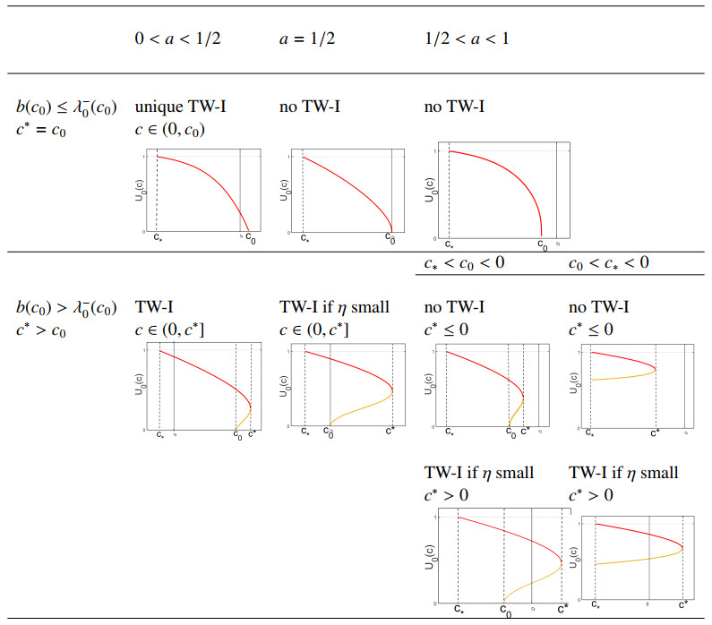
We now use the results from Lemma 7 to study the existence of free traveling waves of type Ⅰ. To study when the free boundary condition (4.1) is satisfied, we consider intersections of the line $ y_1: = c/\alpha \eta_1 $ and the curve $ y_2: = U_0(c) $. The qualitatively different shapes of $ U_0(c) $ are listed in Table 1; the proofs of the (non-) existence of waves are presented in several lemmas. More detailed plots of $ U_0(c) $ with explicit parameter values can be found in [29].
|
 DownLoad:
CSV
DownLoad:
CSV
Lemma 8. If $ 0 < a < 1/2 $ and $ b(c_0)\leq \lambda^-_0(c_0) $, then there exists a unique speed $ c \in (0, c^*) $, for which a free TW-I exists.
Proof. Here, we follow the proof of Theorem 7 in [10]. Since $ b(c_0)\leq \lambda_0^-(c_0) $, we have $ c^* = c_0 $ (Corollary 1). Since $ c > 0 $, we have the existence of a unique forced wave of type Ⅰ for any $ c\in (0, c_0) $ (Section 3.2.1). It remains to show that this solution satisfies (4.1) for a specific value of $ c $ in this interval. At $ c = 0 $, we have $ y_1 = 0 $ and $ y_2 = U_0(0) > 0 $. By part i) of Lemma 7, we know that $ y_2 = U_0(c) $ is continuous and monotone decreasing on $ [0, c^*] $ and $ \lim_{c\to c_0} U_0(c) = 0 $. By the intermediate value theorem, there exists a unique intersection between the line $ y_1 = c/\eta_1\alpha $ and the curve $ y_2 = U_0(c) $, and so (4.1) has a unique solution in $ (0, c_0) $. This solution corresponds to the free traveling wave of type Ⅰ. This case is illustrated in the first column, top row in Table 1.
Lemma 9. If $ 0 < a < 1/2 $ and $ b(c_0) > \lambda^-_0(c_0) $, then there exists at least one speed $ c \in (0, c^*] $, for which a free TW-I exists.
Proof. For this range of parameters, we have $ c_0 < c^* $. By Lemma 7, there are two intersection points, $ U_{0_1}(c) $ and $ U_{0_2}(c), $ with $ U_{0_1}(c^*) = U_{0_2}(c^*) $ and $ U_{0_1}(0) = 0 $; see first column, bottom, in Table 1. Therefore, there is an intersection between one of the curves $ y_2 = U_{0_i}(c) $, $ i = 1, 2 $ and the line $ y_1 = c/\eta_1\alpha $. However, if the line intersects $ U_{0_2}(c) $, there may be more than one intersection, depending on the shape of the $ U_{0_2}(c) $ and the slope of the line.
Lemma 10. For $ a = 1/2 $, we have $ c_0 = 0 $, which leads to the following two cases:
i) If $ b(c_0)\leq \lambda^-_0(c_0) $, or, equivalently, $ \Delta \sqrt{Dm}\geq \frac{\sqrt{2}}{2}, $ then there exists no free TW-I.
ii) If $ b(c_0) > \lambda^-_0(c_0) $, then at least one free TW-I exists for sufficiently small $ \eta_1 > 0 $.
Proof. When $ a = 1/2 $, we have $ c_0 = 0 $. When $ b(c_0)\leq \lambda^-_0(c_0) $, the boundary line is below the tangent line to the heteroclinic connection at $ c_0 = 0 $. Hence, $ U_0(c) $ is monotone decreasing on $ [c_*, 0] $ and $ U_0(0) = 0 $. Therefore, the graph of $ U_0 $ cannot intersect a stright line with positive slope through the origin; see the second column, top plot in Table 1. This proves i).
When $ b(c_0)\leq \lambda^-_0(c_0) $, we have $ c^* > 0 $. By Lemma 7, there are two branches for the intersection point, say, $ U_{0_1}(c) $ and $ U_{0_2}(c) $ with $ U_{0_1}(c^*) = U_{0_2}(c^*) $ and $ U_{0_1}(0) = 0 $; see the second column, bottom plot in Table 1. Therefore, choosing $ \eta_1 $ small enough, the line $ y_1 = c/\eta_1\alpha $ will be steep enough to intersect $ U_{0_i}(c) $, $ i = 1, 2 $ at least once. This intersection corresponds to a free TW-Ⅰ.
When $ 1/2 < a < 1 $, we have $ c_0 < 0 $, so that the maximal speed for forced waves, $ c^* $, can be negative (see Lemma 5). In that case, there is no free TW-Ⅰ because it requires a positive speed. Accordingly, existence, conditional existence, or nonexistence of TW-Ⅰ in this case follows the same ideas as in the proofs of Lemmas 8–10. The results are summarized in the following lemma without proof. The different cases are illustrated in the rightmost column in Table 1.
Lemma 11. For $ 1/2 < a < 1 $,
i) if $ b(c_0)\leq \lambda^-_0(c_0) $, then there exists no free TW-I.
ii) if $ b(c_0) > \lambda^-_0(c_0) $ and $ c^*\leq0 $, then there exists no no free TW-I.
iii) if $ b(c_0) > \lambda^-_0(c_0) $ and $ c^* > 0 $, there exists at least one free TW-I for sufficiently small $ \eta_1 $.
We can express the condition that $ \eta_1 $ be sufficiently small for the existence of traveling waves as follows.
Corollary 2. Let $ a = 1/2 $ (resp., $ 1/2 < a < 1 $). If
|
$ c∗>η1αU0(c∗), $
|
(4.3) |
there is at least one (resp., two) speed(s) in $ (0, c^*) $ for which a TW-I exists.
Proof. If condition (4.3) is satisfied, the line $ y = c/\eta_1\alpha $ lies above the curves $ U_{0_i}(c) $ at $ c^* $, which in turn results in at least one intersection between the two and, hence, a free TW-Ⅰ.
The same geometric considerations in the phase plane as above apply to prove the existence of free TW-Ⅱ in our system for speeds below the maximal speed, $ c^{**} $; see Remark 1. We only summarize the results here.
Corollary 3. If a forced TW-Ⅱ exists (see Theorem 3), it appears for $ c_0 < c\leq c^{**} $ when $ 0 < a\leq1/2 $, and for $ 0 < c \leq c^{**} $ when $ 1/2 < a < 1 $. Then, one can choose $ \eta_1 $ sufficiently small such that there exists at least one free TW-II with (4.1). Otherwise, there exists no free TW-II for scenario 1.
For this scenario, condition (2.23) for the speed of the traveling wave can be written as
|
$ c=η1α(U(0−)−ˉu), $
|
(4.4) |
where $ \bar{u} $ is threshold density at the front. Depending on $ \bar{u} $, the speed can be of any sign, and, hence, the existence of all four types of free waves is possible, but only TW-Ⅰ can appear for any sign of $ c $.
The boundary between advancing and retreating waves are standing waves with $ c = 0 $. We will see that there exist either one or two standing waves depending on the value of $ a $. Therefore, the relative value of $ \bar{u} $ with respect to these standing waves determines the sign of the speed.
We begin by studying forced standing waves with $ c = 0 $ (see [10]). These waves satisfy
|
$ U″+f(U)=0,z<0, $
|
(4.5) |
|
$ U′(0−)=−Δ√DmU(0−), $
|
(4.6) |
|
$ U(−∞)=1. $
|
(4.7) |
This system is conservative with energy function $ E(U, U') = 1/2 (U')^2+F(U) $. We use this to show that the unstable manifold of $ (1, 0) $ intersects the line $ V = -\Delta\sqrt{Dm} U $ corresponding to the boundary condition (4.6). In fact, the orbit that we are looking for satisfies $ E(U(0^-), U'(0^-)) = E(1, 0) $, which, via (4.6), is equivalent to
|
$ m2(α1α2)2D1D2(U′(0−))2+F(U(0−))=F(1). $
|
(4.8) |
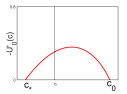
We show that (4.8) has at least one solution; each solution corresponds to a forced TW-Ⅰ.
Lemma 12. i) For $ 0 < a < 1/2 $, there exists a unique value $ 0 < U(0^-) = U_0(0) < 1 $ that satisfies condition (4.8).
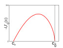
ii) For $ a = 1/2 $, if $ \Delta\sqrt{Dm} \leq \frac{1}{\sqrt{2}} $, then there exists a unique value $ 0 < U(0^-) = U_0(0) < 1 $ that satisfies (4.8).
iii) For $ 1/2 < a < 1 $, if the boundary line $ V = b(0)U $ at $ c = 0 $ lies above the homoclinic connection of $ (1, 0) $ at $ c = 0 $ (resp., is tangent to it), then there exist two values $ 0 < U_{0_2}(0), U_{0_1}(0) < 1 $, (resp., a unique value $ 0 < U_0(0) < 1 $) that satisfies (4.8).
Proof. We follow the idea in Section 3.2. For part $ i) $ (see Figure 7 (a)), when $ 0 < a < 1/2 $, we have $ c_0 > 0 $. Hence, $ M(0) $ lies below the heteroclinic connection of $ (1, 0) $ and $ (0, 0) $ at $ c_0 $ and hits the negative part of the $ V- $axis. On the other hand, as the boundary line $ V = b(0)U $, corresponding to (4.6), has a negative slope, there must be an intersection between $ M(0) $ and $ V = b(0)U $ that satisfies (4.8). One can follow the proof of Theorem 2 and conclude from the direction of the vector field that the intersection is unique.

For part $ ii) $ (see Figure 7 (b)), when $ a = 1/2 $, we have the heteroclinic connection between $ (1, 0) $ and $ (0, 0) $ for $ c_0 = 0 $. To have a unique intersection point $ U_0(0) > 0 $ between the heteroclinic connection and the boundary line $ V = b(0)U $, we follow the idea of Lemma 1 and choose parameters such that the slope of the boundary line is larger than the slope of the heteroclinic connection at $ (0, 0) $. This yields the condition $ -\Delta\sqrt{Dm} \geq \frac{-1}{\sqrt{2}} $.
For part $ iii) $ (see Figure 7(c)), we follow the proof of Lemma 5 (see also Lemma 3.3.10 in [29]). We denote the slope of line that passes through the origin and is tangent to the homoclinic connection of $ (1, 0) $ for $ c = 0 $ as $ \mu $ (see the proof of Lemma 3.3.10 in [29]). Then, if $ b(0) < \mu $, there exists no intersection point between the boundary line and the homoclinic connection satisfying (4.8) and, hence, no standing wave for (4.5)–(4.7). However, if $ b(0) > \mu $ (resp., $ b(0) = \mu $), there exist(s) two (resp., one) intersection(s) between the boundary line and the homoclinic connection satisfying (4.8) and, hence, two (resp., one) standing wave(s) for (4.5)–(4.7).
To study the existence of free TW-Ⅰ with moving boundary condition (4.4), we study the graph of $ U_0(c)-\bar{u} $ with respect to $ c $, which can be found by shifting the graphs in Table 1 downward $ \bar{u} $ units. The intersections of the graphs with the vertical axis in these two figures correspond to $ U_i(0) $ of the standing waves of (4.5)–(4.7), which satisfy (4.8). We summarize the results in Table 2. We refer to Lemma 3.4.11 in [29] for the detailed statements. The corresponding proofs rely on the same geometric considerations as in the preceding lemmas. They are given in the appendix of [29].
| $ \bar{u}=0 $ | $ 0 < \bar{u} < U_0(0) $ | $ \bar{u}=U_0(0) $ | $ U_0(0) < \bar{u} < U_0(c_*) $ | $ \bar{u} > U_0(c_*) $ | |
| $ b(c_0)\leq \lambda_0^-(c_0) $ |  |
Unique TWI | Unique TWI | Unique TWI | Unique TWI |
| if $ \eta $ small | |||||
| $ c^*=c_0 $ | $ c\in(0, c_0) $ | $ c=0 $ | $ c\in(c_*, 0) $ | $ c\in(c_*, 0) $ | |
| $ b(c_0) > \lambda_0^-(c_0) $ |  |
At least one TWI if | Unique TWI | Unique TWI | Unique TWI |
| $ 0 < \bar{u}\leq U_0(c^*) $ | if $ \eta $ small | ||||
| $ c^* > c_0 $ | $ c\in(0, c^*] $ | $ c=0 $ | $ c\in(c_*, 0) $ | $ c\in(c_*, 0) $ | |
| Unique TWI if | |||||
| $ U_0(c^*) < \bar{u} < U_0(c_0) $ | |||||
| $ c\in(0, c^*) $ |
DownLoad:
CSV
Remark 2. The same ideas as for type-I waves can be applied to type-II waves. If a forced TW-II exists (see Theorem 3 for the conditions), we have the following cases, depending on the value of $ a $:
● for $ 0 < a < 1/2 $, if $ 0 < \bar{u}\leq U_{0_1}(c_0) $, then one can choose $ \eta_1 $ such that there exists at least one free TW-II with speed $ c\in (c_0, c^{**}] $ with (4.4). Otherwise, there exists no free TW-II in scenario 2.
● for $ 1/2\leq a < 1 $, if $ 0 < \bar{u}\leq U_{1_0}(0) $, then one can choose $ \eta_1 $ such that there exists at least one free TW-II with speed $ c\in (0, c^{**}] $ with (4.4). Otherwise, there exists no free TW-II in scenario 2.
Remark 3. The situation of free TW-III in scenario 2 is more difficult. As seen in Section 3.2.3, a forced TW-III appears for a specific range of parameters when $ c\in (c_0, c_*) $, and, for a given speed, we may have more than one forced TW-III. One difficulty is that the functions $ U_{0_i}(c) $ for forced TW-III can have quite different shapes, so that the results are not quite as sharp for TW-III as for TW-I. For certain choices of parameters, we can show the existence of free TW-III. For example, if $ c_0\leq c_* $, then for $ \bar{u} > 0 $, one can choose $ \eta_1 $ such that there exists at least one speed $ c \in (c_0, c_*) $ for which a free TW-III exists in scenario. Illustrations can be found in Section 3.4.2 in [29].
The existence of free TW-Ⅳ in scenario 2 can be determined completely. We know from Section 3.2.4 that there exists a forced TW-Ⅳ for all $ c\in (-\infty, c_*) $. Similar to above, one can show that the intersection point $ U_{0}(c) $ for this wave type is a continuous, single-hump function of $ c $ on $ (-\infty, c_*] $, with $ \lim_{c\nearrow c_*}U_0(c) = 1 $, and $ \lim_{c\searrow-\infty}U_{0_1}(c) = 1 $. Given that shape, we cannot expect uniqueness of free TW-Ⅳ, but we obtain their existence (proved similar to Section 4.1).
Lemma 13. For $ 0 < a < 1 $ and $ \bar{u} > 1 $, one can choose $ \eta_1 $ such that there exists at least one speed $ c \in (-\infty, c_*) $ for which we have a free TW-Ⅳ in scenario 2.
We can change our point of view and consider $ \bar u $ and $ c $ as two parameters to obtain free from forced traveling waves. We did this already above when we chose $ c = 0 $ and found values of $ \bar u $ such that corresponding free waves existed. More generally, we can fix $ c $, find a corresponding forced wave (see previous section), and then choose $ \bar u $ so that condition (4.4) is satisfied, which means that we have a free wave of the same type.
Finally, we saw that there can be more than one type of forced wave for a given speed (Figure 4). We can also obtain more than one type of free wave for a given parameter set. For example, Figure 8 shows the curves for $ U_0(c) $ for different types of waves in different colors for $ \bar u = 0 $. Increasing $ \bar u\ne 0 $ will shift the graph down. By choosing $ \eta_1 $ accordingly, the line $ c/(\eta_1 \alpha) $ can intersect the curve at differently colored segments simultaneously. Hence, we can get free waves of different types simultaneously, for example, type Ⅰ (red) and type Ⅲ (currant).

In this scenario, $ B = -\eta_2 U'(0^-) $ and the equation for the speed of the traveling wave is
|
$ c=−η2U′(0−). $
|
(4.9) |
By the assumptions for scenario 3, we have $ U'(0^-) < 0 $ so that the speed must be positive. Therefore, only waves of type Ⅰ and II may occur. We treat this scenario similar to scenario 1 in Section 4.1. Similar to Remark 4.2, we define $ U'_0(c): = U'(0^-) = V(0^-) $ to denote the dependence of $ U'(0^-) $ on $ c $ and use $ U'_{0_i}(c): = U'_i(0^-) $ for $ i = 1, ..., k, $ when we want to denote the $ k $ forced waves corresponding to the same speed $ c $. We investigate the shape of the functions $ U'_0(c) $ in the following lemma and summarize its findings and their implications for the existence of free TW-Ⅰ in Table 3.
| $ 0 < a < 1/2 $ | $ a=1/2 $ | $ 1/2 < a < 1 $ | ||
| $ b(c_0)\leq \lambda_0^-(c_0) $ | unique TWI | no TWI | no TWI | |
| $ c^*=c_0 $ | $ c\in(0, c_0) $ | |||
 |
 |
 |
||
| $ c_* < c_0 < 0 $ | $ c_0 < c_* < 0 $ | |||
| $ b(c_0) > \lambda_0^-(c_0) $ | TWI | TWI if $ \eta $ small | no TWI | no TWI |
| $ c^* > c_0 $ | $ c\in(0, c^*] $ | $ c\in(0, c^*] $ | $ c^*\leq 0 $ | $ c^*\leq 0 $ |
 |
 |
 |
 |
|
| TWI if $ \eta $ small | TWI if $ \eta $ small | |||
| $ c^* > 0 $ | $ c^* > 0 $ | |||
 |
 |
|||
DownLoad:
CSV
Lemma 14. Consider a forced TW-I with $ 0 < a < 1 $ and different values of $ c $. The functions $ -U'_{0_i}(c) $, with $ i = 1, 2 $, have the fallowing properties:
i) If $ b(c_0)\leq \lambda_0(c_0) $, then $ -U'_0(c) $ is a continuous function of $ c $ on $ c_*\leq c \leq c_0 $, $ \lim_{c\nearrow c_0}U'_0(c) = 0 $, and $ \lim_{c\searrow c_*}U'_0(c) = 0 $.
ii) If $ b(c_0) > \lambda_0(c) $, then we have the following properties for $ -U'_{0_1}(c) $ and $ -U'_{0_2}(c) $:
ii-a) $ -U'_{0_1}(c) $ is a continuous function on $ c_*\leq c \leq c^* $, $ \lim_{c\searrow c_*}U'_{0_1}(c) = 0 $, and $ \lim_{c\nearrow c^*}U'_{0_1}(c) = U'_0(c^*) $.
ii-b) If $ c_0\geq c_* $, then $ -U'_{0_2}(c) $ is monotone increasing on $ c_0 < c\leq c^* $, $ \lim_{c\searrow c_0}U'_{0_2}(c) = 0 $, and $ \lim_{c\nearrow c^*}U'_{0_2}(c) = U'_0(c^*) $.
ii-c) If $ c_* > c_0 $, then $ -U'_{0_2}(c) $ is monotone increasing on $ c_*\leq c\leq c^* $, $ \lim_{c\searrow c_*}U'_{0_2}(c) = 0 $, and $ \lim_{c\nearrow c^*}U'_{0_2}(c) = U'_0(c^*) $.
Proof. The proof of this lemma follows the ideas in the proof of Lemma 7. Details can be found in the proof of Lemma 3.4.17 in [29]
To obtain the existence of free TW-Ⅰ from the preceding lemma, one can equivalently prove the existence of at least one intersection between the line $ y = c/\alpha \eta_1 $ and the curves for $ -U'_0(c) $. We consider the different cases with respect to the value of $ a $ as in Section 4.1. Although the graphs of $ -U'_0(c) $ are not exactly the same as the analogous ones for $ U_0(c) $ in the preceding sections, the steps to prove the existence of an intersection are very similar to Section 4.1. Instead of listing all the cases, we simply indicate the result together with the graphs of $ -U'_0(c) $ in Table 3. Detailed formulations of the results can be found in [29].
Again, the existence of free TW-Ⅱ can be treated similarly to that of TW-Ⅰ. We remark without proof that if a forced TW-Ⅱ exists (see Theorem 3 for the conditions), it appears for $ c_0 < c\leq c^{**} $ when $ 0 < a\leq1/2 $, and for $ 0 < c \leq c^{**} $ when $ 1/2 < a < 1 $. Then, one can choose $ \eta_1 $ such that there exists at least one free TW-Ⅱ in (4.9). Otherwise, there exists no TW-Ⅱ for the full system with scenario 3.
Summary: In this section, we studied the existence of free traveling waves, i.e., solutions of the free boundary problem (2.17)–(2.23). Conceptually, the existence condition is not too difficult: it reduces to finding an intersection between a certain curve and a straight line. In practice, however, the proofs become very subtle because the curve is given only implicitly and because there are so many different forms of waves, different scenarios for the interface matching, and so many parameters. The most complete case is scenario 1 for wave type Ⅰ; see Table 1. There are three qualitatively different cases: a unique intersection, no intersection, and a possible intersection or two when the slope of the line is steep enough. The second scenario is still relatively complete for type Ⅰ, II, and IV waves, but the case of type-ⅡI waves is much more difficult. For scenario 3, we only outline the results here since they consist of essentially the same type of considerations and proofs as the previous cases, but are, again, long and tedious.
Classical models for the spatial spread of species are built on relatively simple assumptions of a homogeneous environment whose ability to sustain the spreading species is unaffected by the species itself. Those models support traveling waves of relatively simple shapes: typically, we observe monotone connections between spatially constant steady states [2,40]. When the population dynamics include a strong Allee effect, nonmonotone waves can occur, but they connect two positive states rather than a positive and the zero state [12]; hence, we do not interpret these as the spread of a new species. In systems of multiple populations, their interactions can lead to more complex dynamics in the corresponding nonspatial model, which become visible as oscillatory and chaotic patterns in the wake of an invasion in spatial models [3].
In our work, we discovered and classified multiple novel shapes of traveling waves, based on habitat heterogeneity and an Allee effect. These shapes result from one of two mechanisms: in the case of forced waves, there is an external driver (e.g., climate change) that moves the boundary between suitable and unsuitable habitat. This forced moving boundary, combined with the species' behavioral response (e.g., movement choice) and the Allee effect, lead to four types of traveling waves that can even coexist. This part of our work generalizes the work by Hadeler and Rothe [12] on a homogeneous environment to the case of moving-habitat models. In the case of free waves, the species itself, through its engineering activity, is the driver that moves the boundary between suitable and unsuitable habitat. This part of our work extends previous work by Lutscher, Fink, and Zhu [10], who considered a growth function without Allee effect. Our work differs significantly from other recent attempts of modeling species spread with a free boundary (e.g., [13,17]) in that those authors consider the population to be absent outside of the suitable habitat and use only the third scenario for the movement of the boundary.
While we have shown the existence of a plethora of forced and free traveling waves, the next important step is to consider their stability. This is particularly relevant in the case when there are two or more coexisting waves. We would like to know which of these will manifest for given initial conditions. While preliminary numerical simulations (see Figure 9) indicate that type-Ⅰ waves are frequently observed (and, therefore, expected to be stable), there are subtle distinctions to be made. For example, when there are two TW-Ⅰ for the same speed, which of the two is stable? To fully answer this question is a massive future challenge, in part because there are so many different scenarios and types of waves, and in part because our understanding of the equations with the discontinuous condition at the interface between the two types of habitat is still fairly limited.

Knowledge of which of the traveling wave types are stable and which are unstable would also be the next step in connecting our model and results with ecological theory and observations. Our model is not predictive but rather explorative. We are asking which patterns of spread result from a certain set of assumptions on the movement and engineering behavior of individuals around habitat edges. Which of these individual behaviors can actually be found in which species in nature is a "local'' question: it does not require the observation of traveling waves over large spatiotemporal scales, but only individual behavior localized near an edge of favorable habitat. Once this individual behavior is known or observed, our model and results suggest larger-scale patterns that we should be able to observe.
Actually searching for evidence of such waves in nature is a formidable challenge. This search is made complicated by the fact that we have, necessarily, idealized many aspects in our model. Probably most importantly, we have an abrupt transition from suitable to unsuitable habitat. We expect that this transition is more gradual in nature. What we then need to look for are systems where the dispersal distance of individuals is relatively large to the width of the transition zone between the two environments.
The authors declare that they have not used Artificial Intelligence (AI) tools in the creation of this article.
FL gratefully acknowledges funding from the Natural Sciences and Engineering Research Council of Canada through the Discovery Grants program (RGPIN-2016-04795). The authors thank six reviewers for their valuable input.
The authors declare that there are no conflicts of interest.
Rinaldo M. Colombo, Benedetto Piccoli. Preface[J]. Networks and Heterogeneous Media, 2011, 6(3): i-iii. doi: 10.3934/nhm.2011.6.3i

|
|
DownLoad:
CSV
| $ \bar{u}=0 $ | $ 0 < \bar{u} < U_0(0) $ | $ \bar{u}=U_0(0) $ | $ U_0(0) < \bar{u} < U_0(c_*) $ | $ \bar{u} > U_0(c_*) $ | |
| $ b(c_0)\leq \lambda_0^-(c_0) $ | |
Unique TWI | Unique TWI | Unique TWI | Unique TWI |
| if $ \eta $ small | |||||
| $ c^*=c_0 $ | $ c\in(0, c_0) $ | $ c=0 $ | $ c\in(c_*, 0) $ | $ c\in(c_*, 0) $ | |
| $ b(c_0) > \lambda_0^-(c_0) $ | |
At least one TWI if | Unique TWI | Unique TWI | Unique TWI |
| $ 0 < \bar{u}\leq U_0(c^*) $ | if $ \eta $ small | ||||
| $ c^* > c_0 $ | $ c\in(0, c^*] $ | $ c=0 $ | $ c\in(c_*, 0) $ | $ c\in(c_*, 0) $ | |
| Unique TWI if | |||||
| $ U_0(c^*) < \bar{u} < U_0(c_0) $ | |||||
| $ c\in(0, c^*) $ |
DownLoad:
CSV
| $ 0 < a < 1/2 $ | $ a=1/2 $ | $ 1/2 < a < 1 $ | ||
| $ b(c_0)\leq \lambda_0^-(c_0) $ | unique TWI | no TWI | no TWI | |
| $ c^*=c_0 $ | $ c\in(0, c_0) $ | |||
|
|
|
||
| $ c_* < c_0 < 0 $ | $ c_0 < c_* < 0 $ | |||
| $ b(c_0) > \lambda_0^-(c_0) $ | TWI | TWI if $ \eta $ small | no TWI | no TWI |
| $ c^* > c_0 $ | $ c\in(0, c^*] $ | $ c\in(0, c^*] $ | $ c^*\leq 0 $ | $ c^*\leq 0 $ |
|
|
|
|
|
| TWI if $ \eta $ small | TWI if $ \eta $ small | |||
| $ c^* > 0 $ | $ c^* > 0 $ | |||
|
|
|||
DownLoad:
CSV
|
|
| $ \bar{u}=0 $ | $ 0 < \bar{u} < U_0(0) $ | $ \bar{u}=U_0(0) $ | $ U_0(0) < \bar{u} < U_0(c_*) $ | $ \bar{u} > U_0(c_*) $ | |
| $ b(c_0)\leq \lambda_0^-(c_0) $ | |
Unique TWI | Unique TWI | Unique TWI | Unique TWI |
| if $ \eta $ small | |||||
| $ c^*=c_0 $ | $ c\in(0, c_0) $ | $ c=0 $ | $ c\in(c_*, 0) $ | $ c\in(c_*, 0) $ | |
| $ b(c_0) > \lambda_0^-(c_0) $ | |
At least one TWI if | Unique TWI | Unique TWI | Unique TWI |
| $ 0 < \bar{u}\leq U_0(c^*) $ | if $ \eta $ small | ||||
| $ c^* > c_0 $ | $ c\in(0, c^*] $ | $ c=0 $ | $ c\in(c_*, 0) $ | $ c\in(c_*, 0) $ | |
| Unique TWI if | |||||
| $ U_0(c^*) < \bar{u} < U_0(c_0) $ | |||||
| $ c\in(0, c^*) $ |
| $ 0 < a < 1/2 $ | $ a=1/2 $ | $ 1/2 < a < 1 $ | ||
| $ b(c_0)\leq \lambda_0^-(c_0) $ | unique TWI | no TWI | no TWI | |
| $ c^*=c_0 $ | $ c\in(0, c_0) $ | |||
|
|
|
||
| $ c_* < c_0 < 0 $ | $ c_0 < c_* < 0 $ | |||
| $ b(c_0) > \lambda_0^-(c_0) $ | TWI | TWI if $ \eta $ small | no TWI | no TWI |
| $ c^* > c_0 $ | $ c\in(0, c^*] $ | $ c\in(0, c^*] $ | $ c^*\leq 0 $ | $ c^*\leq 0 $ |
|
|
|
|
|
| TWI if $ \eta $ small | TWI if $ \eta $ small | |||
| $ c^* > 0 $ | $ c^* > 0 $ | |||
|
|
|||
