We present a new comprehensive mathematical model of the cone-shaped cantilever tip-sample interaction in Atomic Force Microscopy (AFM). The importance of such AFMs with cone-shaped cantilevers can be appreciated when its ability to provide high-resolution information at the nanoscale is recalled. It is an indispensable tool in a wide range of scientific and industrial fields. The interaction of the cone-shaped cantilever tip with the surface of the specimen (sample) is modeled by the damped Euler-Bernoulli beam equation $ \rho_A(x)u_{tt} $ $ +\mu(x)u_{t}+(r(x)u_{xx}+\kappa(x)u_{xxt})_{xx} = 0 $, $ (x, t)\in (0, \ell)\times (0, T) $, subject to the following initial, $ u(x, 0) = 0 $, $ u_t(x, 0) = 0 $ and boundary, $ u(0, t) = 0 $, $ u_{x}(0, t) = 0 $, $ \left (r(x)u_{xx}(x, t)+\kappa(x)u_{xxt} \right)_{x = \ell} = M(t) $, $ \left (-(r(x)u_{xx}+\kappa(x)u_{xxt})_x\right)_{x = \ell} = g(t) $ conditions, where $ M(t): = 2h\cos \theta\, g(t)/\pi $ is the moment generated by the transverse shear force $ g(t) $. Based on this model, we propose an inversion algorithm for the reconstruction of an unknown shear force in the AFM cantilever. The measured displacement $ \nu(t): = u(\ell, t) $ is used as additional data for the reconstruction of the shear force $ g(t) $. The least square functional $ J(F) = \frac{1}{2}\Vert u(\ell, \cdot)-\nu \Vert_{L^2(0, T)}^2 $ is introduced and an explicit gradient formula for the Fréchet derivative of the cost functional is derived via the weak solution of the adjoint problem. Additionally, the geometric parameters of the cone-shaped tip are explicitly contained in this formula. This enables us to construct a gradient based numerical algorithm for the reconstructions of the shear force from noise free as well as from random noisy measured output $ \nu (t) $. Computational experiments show that the proposed algorithm is very fast and robust. This creates the basis for developing a numerical "gadget" for computational experiments with generic AFMs.
Citation: Alemdar Hasanov, Alexandre Kawano, Onur Baysal. Reconstruction of shear force in Atomic Force Microscopy from measured displacement of the cone-shaped cantilever tip[J]. Mathematics in Engineering, 2024, 6(1): 137-154. doi: 10.3934/mine.2024006
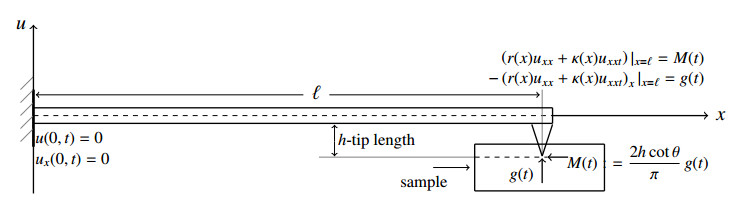
We present a new comprehensive mathematical model of the cone-shaped cantilever tip-sample interaction in Atomic Force Microscopy (AFM). The importance of such AFMs with cone-shaped cantilevers can be appreciated when its ability to provide high-resolution information at the nanoscale is recalled. It is an indispensable tool in a wide range of scientific and industrial fields. The interaction of the cone-shaped cantilever tip with the surface of the specimen (sample) is modeled by the damped Euler-Bernoulli beam equation $ \rho_A(x)u_{tt} $ $ +\mu(x)u_{t}+(r(x)u_{xx}+\kappa(x)u_{xxt})_{xx} = 0 $, $ (x, t)\in (0, \ell)\times (0, T) $, subject to the following initial, $ u(x, 0) = 0 $, $ u_t(x, 0) = 0 $ and boundary, $ u(0, t) = 0 $, $ u_{x}(0, t) = 0 $, $ \left (r(x)u_{xx}(x, t)+\kappa(x)u_{xxt} \right)_{x = \ell} = M(t) $, $ \left (-(r(x)u_{xx}+\kappa(x)u_{xxt})_x\right)_{x = \ell} = g(t) $ conditions, where $ M(t): = 2h\cos \theta\, g(t)/\pi $ is the moment generated by the transverse shear force $ g(t) $. Based on this model, we propose an inversion algorithm for the reconstruction of an unknown shear force in the AFM cantilever. The measured displacement $ \nu(t): = u(\ell, t) $ is used as additional data for the reconstruction of the shear force $ g(t) $. The least square functional $ J(F) = \frac{1}{2}\Vert u(\ell, \cdot)-\nu \Vert_{L^2(0, T)}^2 $ is introduced and an explicit gradient formula for the Fréchet derivative of the cost functional is derived via the weak solution of the adjoint problem. Additionally, the geometric parameters of the cone-shaped tip are explicitly contained in this formula. This enables us to construct a gradient based numerical algorithm for the reconstructions of the shear force from noise free as well as from random noisy measured output $ \nu (t) $. Computational experiments show that the proposed algorithm is very fast and robust. This creates the basis for developing a numerical "gadget" for computational experiments with generic AFMs.

| [1] | M. Antognozzi, Investigation of the shear force contrast mechanism in transverse dynamic force microscopy, Ph.D. Thesis, University of Bristol, UK, 2000. |
| [2] |
M. Antognozzi, D. R. Binger, A. D. L. Humphris, P. J. James, M. J. Miles, Modeling of cylindrically tapered cantilevers for transverse dynamic force microscopy (TDFM), Ultramicroscopy, 86 (2001), 223–232. https://doi.org/10.1016/S0304-3991(00)00087-5 doi: 10.1016/S0304-3991(00)00087-5

|
| [3] |
H. T. Banks, D. J. Inman, On damping mechanisms in beams, J. Appl. Mech., 58 (1991), 716–723. https://doi.org/10.1115/1.2897253 doi: 10.1115/1.2897253
|
| [4] |
G. Binnig, C. F. Quate, C. Gerber, Atomic force microscopy, Phys. Rev. Lett., 56 (1986), 930. https://doi.org/10.1103/PhysRevLett.56.930 doi: 10.1103/PhysRevLett.56.930
|
| [5] |
W. J. Chang, T. H. Fang, C. I. Weng, Inverse determination of the cutting force on nanoscale processing using atomic force microscopy, Nanotechnology, 15 (2004), 427–430. https://doi.org/10.1088/0957-4484/15/5/004 doi: 10.1088/0957-4484/15/5/004
|
| [6] | L. C. Evans, Partial differential equations, 2 Eds., Providence: American Mathematical Society, 2010. |
| [7] |
B. Geist, J. R. McLaughlin, The effect of structural damping on nodes for the Euler-Bernoulli beam: a specific case study, Appl. Math. Lett., 7 (1994), 51–55. https://doi.org/10.1016/0893-9659(94)90112-0 doi: 10.1016/0893-9659(94)90112-0
|
| [8] |
A. Hasanov, O. Baysal, Identification of an unknown spatial load distribution in a vibrating cantilever beam from final overdetermination, J. Inverse Ill-Posed Probl., 23 (2015), 85–102. https://doi.org/10.1515/jiip-2014-0010 doi: 10.1515/jiip-2014-0010
|
| [9] |
A. Hasanov, O. Baysal, Identification of unknown temporal and spatial load distributions in a vibrating Euler-Bernoulli beam from Dirichlet boundary measured data, Automatica, 71 (2016), 106–117. https://doi.org/10.1016/j.automatica.2016.04.034 doi: 10.1016/j.automatica.2016.04.034
|
| [10] |
A. Hasanov, O. Baysal, C. Sebu, Identification of an unknown shear force in the Euler-Bernoulli cantilever beam from measured boundary deflection, Inverse Probl., 35 (2019), 115008. https://doi.org/10.1088/1361-6420/ab2a34 doi: 10.1088/1361-6420/ab2a34
|
| [11] |
A. Hasanov, O. Baysal, H. Itou, Identification of an unknown shear force in a cantilever Euler-Bernoulli beam from measured boundary bending moment, J. Inverse Ill-posed Probl., 27 (2019), 859–876. https://doi.org/10.1515/jiip-2019-0020 doi: 10.1515/jiip-2019-0020
|
| [12] | A. H. Hasanoglu, A. G. Romanov, Introduction to inverse problems for differential equations, 2 Eds., New York: Springer, 2021. |
| [13] | G. Haugstad, Atomic force microscopy: understanding basic modes and advanced applications, Wiley, 2012. |
| [14] |
O. Baysal, A. Hasanov, K. Sakthivel, Determination of unknown shear force in transverse dynamic force microscopy from measured final data, J. Inverse Ill-posed Probl., 2023. https://doi.org/10.1515/jiip-2023-0021 doi: 10.1515/jiip-2023-0021
|
| [15] |
S. Kumarasamy, A. Hasanov, A. Dileep, Inverse problems of identifying the unknown transverse shear force in the Euler-Bernoulli beam with Kelvin-Voigt damping, J. Inverse Ill-posed Probl., 2023. https://doi.org/10.1515/jiip-2022-0053 doi: 10.1515/jiip-2022-0053
|
| [16] |
H. L. Lee, W. J. Chang, Effects of damping on the vibration frequency of atomic force microscope cantilevers using the Timoshenko beam model, Jpn. J. Appl. Phys., 48 (2009), 065005. https://doi.org/10.1143/JJAP.48.065005 doi: 10.1143/JJAP.48.065005
|
| [17] |
J. S. Lee, J. Song, S. O. Kim, S. Kim, W. Lee, J. A. Jackman, et al., Multifunctional hydrogel nano-probes for atomic force microscopy, Nat. Commun., 7 (2016), 11566. https://doi.org/10.1038/ncomms11566 doi: 10.1038/ncomms11566
|
| [18] |
M. P. Scherer, G. Frank, A. W. Gummer, Experimental determination of the mechanical impedance of atomic force microscopy cantilevers in fluids up to $70$ kHz, J. Appl. Phys., 88 (2000), 2912–2920. https://doi.org/10.1063/1.1287522 doi: 10.1063/1.1287522
|
| [19] |
K. Shen, D. C. Hurley, J. A. Turner, Dynamic behaviour of dagger-shaped cantilevers for atomic force microscopy, Nanotechnology, 15 (2004), 1582–1589. https://doi.org/10.1088/0957-4484/15/11/036 doi: 10.1088/0957-4484/15/11/036
|
| [20] |
J. A. Turner, J. S. Wiehn, Sensitivity of flexural and torsional vibration modes of atomic force microscope cantilevers to surface stiffness variations, Nanotechnology, 12 (2001), 322–330. https://doi.org/10.1088/0957-4484/12/3/321 doi: 10.1088/0957-4484/12/3/321
|
| [21] |
N. R. Wilson, J. V. Macpherson, Carbon nanotube tips for atomic force microscopy, Nature Nanotechnology, 4 (2009), 483–491. https://doi.org/10.1038/nnano.2009.154 doi: 10.1038/nnano.2009.154
|
| [22] |
K. Zhang, T. Nguyen, C. Edwards, M. Antognozzi, M. Miles, G. Herrmann, Real-time force reconstruction in a transverse dynamic force microscope, IEEE Trans. Ind. Electron., 69 (2022), 11403–11413. https://doi.org/10.1109/TIE.2021.3120487 doi: 10.1109/TIE.2021.3120487
|


Figures(5)

Alemdar Hasanov, Alexandre Kawano, Onur Baysal. Reconstruction of shear force in Atomic Force Microscopy from measured displacement of the cone-shaped cantilever tip[J]. Mathematics in Engineering, 2024, 6(1): 137-154. doi: 10.3934/mine.2024006


 DownLoad: