This work presents models for homogenizing or finding the effective transport or mechanical properties of microscale composites formed from highly contrasting phases described on a grid. The methods developed here are intended for engineering applications where speed and geometrical flexibility are a premium. A canonical case that is mathematically challenging and yet can be applied to many realistic materials is a 4-phase 2-dimensional periodic checkerboard or tiling. While analytic solutions for calculating effective properties exist for some cases, versatile methods are needed to handle anisotropic and non-square grids. A reinterpretation and extension of an existing analytic solution that utilizes equivalent circuits is developed. The resulting closed-form expressions for effective conductivity are shown to be accurate within a few percent or better for multiple cases of interest. Secondly a versatile and efficient spectral method is presented as a solution to the 4-phase primitive cell with a variety of external boundaries. The spectral method expresses the solution to effective conductivity in terms of analytically derived eigenfunctions and numerically determined spectral coefficients. The method is validated by comparing to known solutions and can allow extensions to cases with no current analytic solution.
Citation: Ben J. Ransom, Dean R. Wheeler. Rapid computation of effective conductivity of 2D composites by equivalent circuit and spectral methods[J]. Mathematics in Engineering, 2022, 4(3): 1-24. doi: 10.3934/mine.2022020
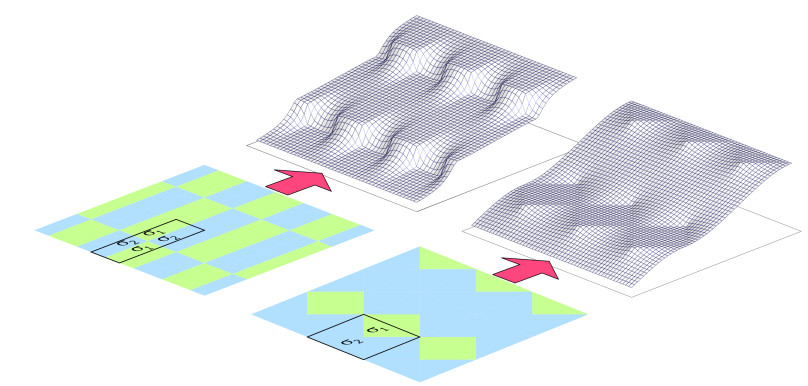
This work presents models for homogenizing or finding the effective transport or mechanical properties of microscale composites formed from highly contrasting phases described on a grid. The methods developed here are intended for engineering applications where speed and geometrical flexibility are a premium. A canonical case that is mathematically challenging and yet can be applied to many realistic materials is a 4-phase 2-dimensional periodic checkerboard or tiling. While analytic solutions for calculating effective properties exist for some cases, versatile methods are needed to handle anisotropic and non-square grids. A reinterpretation and extension of an existing analytic solution that utilizes equivalent circuits is developed. The resulting closed-form expressions for effective conductivity are shown to be accurate within a few percent or better for multiple cases of interest. Secondly a versatile and efficient spectral method is presented as a solution to the 4-phase primitive cell with a variety of external boundaries. The spectral method expresses the solution to effective conductivity in terms of analytically derived eigenfunctions and numerically determined spectral coefficients. The method is validated by comparing to known solutions and can allow extensions to cases with no current analytic solution.

| [1] | G. Milton, The theory of composites, Cambridge: Cambridge University Press, 2002. |
| [2] |
S. Torquato, Optimal design of heterogeneous materials, Annu. Rev. Mater. Res., 40 (2010), 101-129. doi: 10.1146/annurev-matsci-070909-104517

|
| [3] |
D. Felbacq, G. Bouchitte, Homogenization of a set of parallel fibres, Waves in Random Media, 7 (1997), 245-256. doi: 10.1088/0959-7174/7/2/006
|
| [4] |
G. Milton, Proof of a conjecture on the conductivity of checkerboards, J. Math Phys., 42 (2001), 4873-4882. doi: 10.1063/1.1385564
|
| [5] |
M. Karim, K. Krabbenhoft, New renormalization schemes for conductivity upscaling in heterogeneous media, Transport Porous Med., 85 (2010), 677-690. doi: 10.1007/s11242-010-9585-9
|
| [6] |
W. Suen, S. Wong, K. Young, The lattice model of heat conduction in a composite material, J. Phys. D Appl. Phys., 12 (1979), 1325-1338. doi: 10.1088/0022-3727/12/8/013
|
| [7] | S. A. Berggren, D. Lukkassen, A. Meidell, L. Simula, A new method for numerical solution of checkerboard fields, J. Appl. Math., 1 (2001), 615091. |
| [8] |
J. Bigalke, Derivation of an equation to calculate the average conductivity of random networks, Physica A, 285 (2000), 295-305. doi: 10.1016/S0378-4371(00)00262-4
|
| [9] |
D. Yushu, K. Matouš, The image-based multiscale multigrid solver, preconditioner, and reduced order model, J. Comput. Phys., 406 (2020), 109165. doi: 10.1016/j.jcp.2019.109165
|
| [10] |
L. Zielke, T. Hutzenlaub, D. Wheeler, C. W. Chao, I. Manke, A. Hilger, et al., Three-phase multiscale modeling of a LiCoO2 cathode: Combining the advantages of FIB-SEM imaging and X-ray tomography, Adv. Energy Mater., 5 (2015), 1401612. doi: 10.1002/aenm.201401612
|
| [11] | D. E. Stephenson, B. C. Walker, C. B. Skelton, E. Gorzkowski, Modeling 3D microstructure and ion transport in porous Li-ion battery electrodes, J. Electrochem. Soc., 158 (2011): A781-A789. |
| [12] |
L. Jylha, A. Sihvola, Approximations and full numerical simulations for the conductivity of three dimensional checkerboard geometries, IEEE T. Dielect. El. In., 13 (2006), 760-764. doi: 10.1109/TDEI.2006.1667733
|
| [13] |
J. Helsing, The effective conductivity of random checkerboards, J. Comput. Phys., 230 (2011), 1171-1181. doi: 10.1016/j.jcp.2010.10.033
|
| [14] |
R. Edwards, J. Goodman, A. Sokal, Multigrid method for the random-resistor problem, Phys. Rev. Lett., 61 (1988), 1333-1335. doi: 10.1103/PhysRevLett.61.1333
|
| [15] |
S. Torquato, I. Kim, D. Cule, Effective conductivity, dielectric constant, and diffusion coefficient of digitized composite media via first-passage-time equations, J. Appl. Phys., 85 (1999), 1560-1571. doi: 10.1063/1.369287
|
| [16] |
S. S. Wei, J. S. Shen, W. Y. Yang, Z. L. Li, S. H. Di, C. Ma, Application of the renormalization group approach for permeability estimation in digital rocks, J. Petrol. Sci. Eng., 179 (2019), 631-644. doi: 10.1016/j.petrol.2019.04.057
|
| [17] | P. King, Upscaling permeability: Error analysis for renormalization, Transport Porous Med., 23 (1996), 337-354. |
| [18] | S. Mortola, S. Steffé, A two-dimensional homogenization problem, Atti Accad. Naz. Lincei Rend. Cl. Sci. Fis. Mat. Natur., 78 (1985), 77-82. |
| [19] |
R. Craster, Y. Obnosov, Four-phase checkerboard composites, SIAM J. Appl. Math., 61 (2001), 1839-1856. doi: 10.1137/S0036139900371825
|
| [20] |
J. Keller, A theorem on the conductivity of a composite medium, J. Math. Phys., 5 (1964), 548-549. doi: 10.1063/1.1704146
|
| [21] | J. Maxwell, A treatise on electricity and magnetism, 2 Eds., Oxford: Cambridge, 1881,398-411. |
| [22] |
J. Keller, Effective conductivity of periodic composites composed of two very unequal conductors, J. Math. Phys., 28 (1987), 2516-2520. doi: 10.1063/1.527741
|
| [23] | R. Craster, Y. Obnosov, A model four-phase square checkerboard structure, Q. J. Mech. Appl. Math., 59 (2006), 20-23. |
| [24] |
R. Craster, R. Obnosov, A three-phase tessellation: Solution and effective properties, Proc. R. Soc. Lond. A, 460 (2004), 1017-1037. doi: 10.1098/rspa.2003.1196
|
| [25] |
J. Helsing, Corner singularities for elliptic problems: special basis functions versus 'brute force', Commun. Numer. Meth. Eng., 16 (2000), 37-46. doi: 10.1002/(SICI)1099-0887(200001)16:1<37::AID-CNM307>3.0.CO;2-1
|
| [26] | T. Choy, Effective medium theory, Oxford: Clarendon Press, 1999. |
| [27] | A. Dykhne, Conductivity of a two-dimensional two-phase system, Soviet Journal of Experimental and Theoretical Physics, 32 (1971), 63. |


Figures(14)

Ben J. Ransom, Dean R. Wheeler. Rapid computation of effective conductivity of 2D composites by equivalent circuit and spectral methods[J]. Mathematics in Engineering, 2022, 4(3): 1-24. doi: 10.3934/mine.2022020


 DownLoad: