4q interstitial and terminal deletion: clinical features comparison in two unrelated children

Piero Pavone; Xena Giada Pappalardo; Riccardo Lubrano; Salvatore Savasta; Alberto Verrotti; Pasquale Parisi; Raffaele Falsaperla; Piero Pavone; Xena Giada Pappalardo; Riccardo Lubrano; Salvatore Savasta; Alberto Verrotti; Pasquale Parisi; Raffaele Falsaperla

doi:10.3934/medsci.2023011

AIMS Medical Science

2023, Volume 10, Issue 2: 130-140. doi: 10.3934/medsci.2023011

Previous Article Next Article

Case report

4q interstitial and terminal deletion: clinical features comparison in two unrelated children

1.
Section of Pediatrics and Child Neuropsychiatry, Department of Child and Experimental Medicine, University of Catania, Italy
2.
National Council of Research, Institute for Biomedical Research and Innovation (IRIB), Unit of Catania, Italy
3.
Department of Biomedical and Biotechnological Sciences (BIOMETEC), University of Catania, Italy
4.
Department of Pediatrics, Sapienza University of Rome, Pediatric and Neonatology Unit, Hospital Goretti Polo Pontino, Rome, Italy
5.
Department of Pediatrics, University of Cagliari, Pediatric and Neonatology Unit, Cagliari, Italy
6.
Pediatric Clinic, Department of Medicine, University of Perugia, 06129 Perugia, Italy
7.
Child Neurology, NESMOS Department, Faculty of Medicine & Psychology, Sapienza University of Rome, Rome, Italy
8.
Pediatric and Pediatric Emergency Department, University Hospital, A.U.O “Policlinico Vittorio Emanuele”, Catania, Italy
† These two authors contributed equally.

Received: 04 January 2023 Revised: 24 April 2023 Accepted: 11 May 2023 Published: 26 May 2023

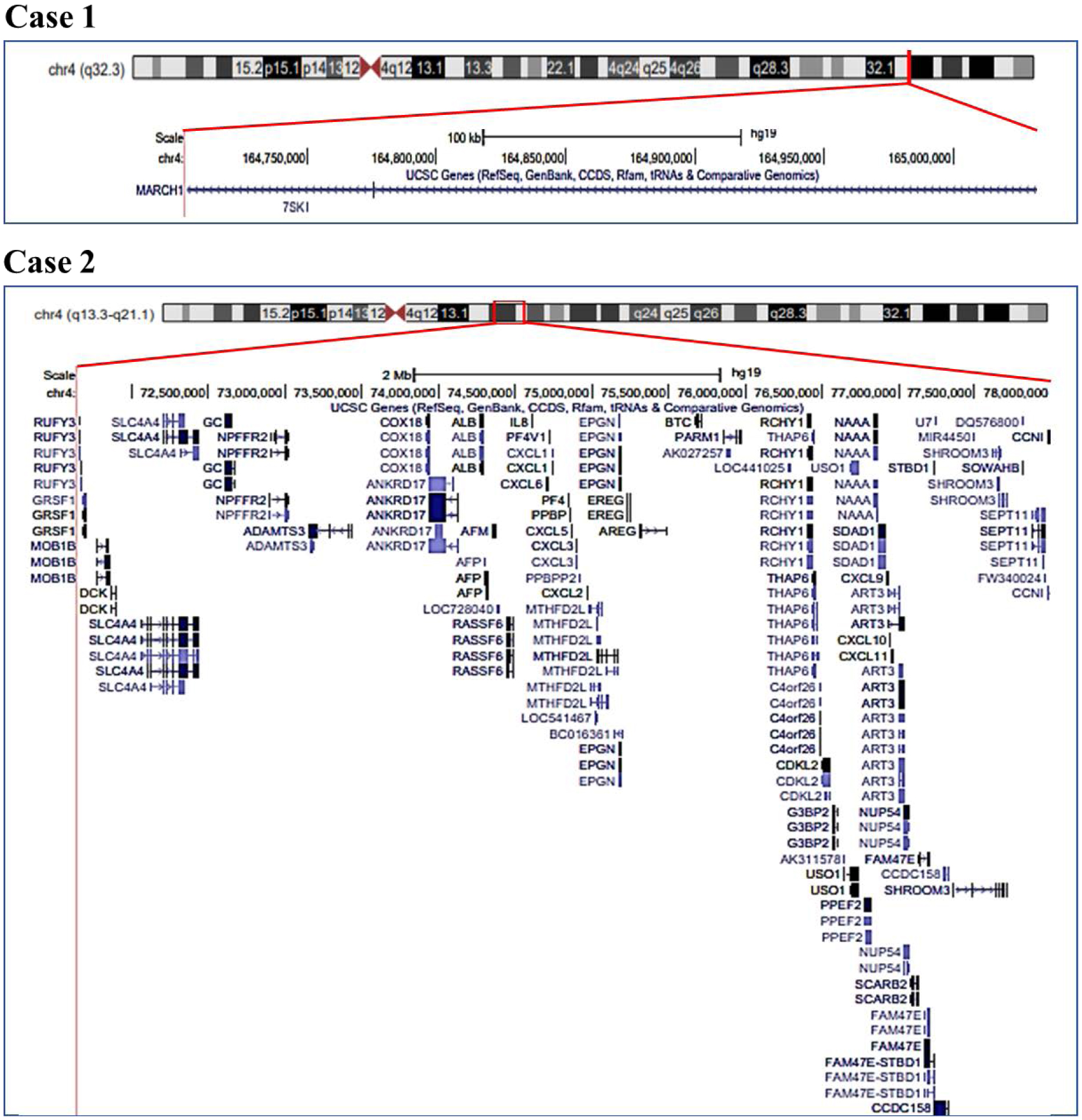
The 4q deletion syndrome defines a disorder, which may involve patients affected by either the deletion of the interstitial region from the centromere to 4q31 or by the deletion of the terminal region from 4q31 to 4qter. Here, we describe clinical phenotypes of two unrelated children of the same age followed at the same time, with case 1 presenting with 4q interstitial and case 2 with terminal 4q deletion, and compare them each other and with those reported in the literature. Both children showed complex, heterogeneous clinical manifestations, including craniofacial features, pre-postnatal growth failure, speech and developmental delay. In case 2, thyroid and cholesterol dysfunction were also found. Analyzing these data, clinical differences between interstitial and terminal 4q deletions are scanty and no significant phenotype differences were found between the 4q regions deleted as observed in the comparison of the two children and the related cases of the literature. The term 4q deletion syndrome - inclusive for both the interstitial and terminal 4q regions deleted - seems to be appropriate. To note, the dysfunction of cholesterol metabolism and thyroid presented by case 2 may be clinically worthwhile, whether confirmed by other observations.

Keywords:

4q deletion syndrome,
terminal 4q deletion,
interstitial 4q deletion,
craniofacial malformations,
developmental delay/intellectual disability (DD/ID)

Citation: Piero Pavone, Xena Giada Pappalardo, Riccardo Lubrano, Salvatore Savasta, Alberto Verrotti, Pasquale Parisi, Raffaele Falsaperla. 4q interstitial and terminal deletion: clinical features comparison in two unrelated children[J]. AIMS Medical Science, 2023, 10(2): 130-140. doi: 10.3934/medsci.2023011

Related Papers:

[1]	Wei Lu, Yuangang Li, Yixiu Kong, Liangli Yang . Generalized triangular Pythagorean fuzzy weighted Bonferroni operators and their application in multi-attribute decision-making. AIMS Mathematics, 2023, 8(12): 28376-28397. doi: 10.3934/math.20231452
[2]	Tahir Mahmood, Azam, Ubaid ur Rehman, Jabbar Ahmmad . Prioritization and selection of operating system by employing geometric aggregation operators based on Aczel-Alsina t-norm and t-conorm in the environment of bipolar complex fuzzy set. AIMS Mathematics, 2023, 8(10): 25220-25248. doi: 10.3934/math.20231286
[3]	Tahir Mahmood, Ubaid Ur Rehman, Muhammad Naeem . A novel approach towards Heronian mean operators in multiple attribute decision making under the environment of bipolar complex fuzzy information. AIMS Mathematics, 2023, 8(1): 1848-1870. doi: 10.3934/math.2023095
[4]	Weiwei Jiang, Zeeshan Ali, Muhammad Waqas, Peide Liu . Decision methods based on Bonferroni mean operators and EDAS for the classifications of circular pythagorean fuzzy Meta-analysis. AIMS Mathematics, 2024, 9(10): 28273-28294. doi: 10.3934/math.20241371
[5]	Shichao Li, Zeeshan Ali, Peide Liu . Prioritized Hamy mean operators based on Dombi t-norm and t-conorm for the complex interval-valued Atanassov-Intuitionistic fuzzy sets and their applications in strategic decision-making problems. AIMS Mathematics, 2025, 10(3): 6589-6635. doi: 10.3934/math.2025302
[6]	Muhammad Qiyas, Muhammad Naeem, Neelam Khan, Lazim Abdullah . Bipolar complex fuzzy credibility aggregation operators and their application in decision making problem. AIMS Mathematics, 2023, 8(8): 19240-19263. doi: 10.3934/math.2023981
[7]	Dilshad Alghazzawi, Sajida Abbas, Hanan Alolaiyan, Hamiden Abd El-Wahed Khalifa, Alhanouf Alburaikan, Qin Xin, Abdul Razaq . Dynamic bipolar fuzzy aggregation operators: A novel approach for emerging technology selection in enterprise integration. AIMS Mathematics, 2024, 9(3): 5407-5430. doi: 10.3934/math.2024261
[8]	Anam Habib, Zareen A. Khan, Nimra Jamil, Muhammad Riaz . A decision-making strategy to combat CO$ _2 $ emissions using sine trigonometric aggregation operators with cubic bipolar fuzzy input. AIMS Mathematics, 2023, 8(7): 15092-15128. doi: 10.3934/math.2023771
[9]	Khulud Fahad Bin Muhaya, Kholood Mohammad Alsager . Extending neutrosophic set theory: Cubic bipolar neutrosophic soft sets for decision making. AIMS Mathematics, 2024, 9(10): 27739-27769. doi: 10.3934/math.20241347
[10]	Asit Dey, Tapan Senapati, Madhumangal Pal, Guiyun Chen . A novel approach to hesitant multi-fuzzy soft set based decision-making. AIMS Mathematics, 2020, 5(3): 1985-2008. doi: 10.3934/math.2020132

Abstract

Abbreviations: FST: Fuzzy set theory; BFST: Bipolar fuzzy set theory; CFST: Complex fuzzy set theory; BCFST: Bipolar complex fuzzy set theory; BM: Bonferroni mean; BCFBM: Bipolar complex fuzzy Bonferroni mean; BCFNWBM: Bipolar complex fuzzy normalized weighted Bonferroni mean; BCFOWBM: Bipolar complex fuzzy ordered weighted Bonferroni mean; MADM: Multiattribute decision-making; SG: Supporting grade

1. Introduction

In mathematics, the decision-making technique is the procedure of expressing real life problems and events in a mathematical and statistical format or language. Many techniques exist in the field of mathematics and are used for evaluating or carrying out mathematical and statistical problems and one of these techniques is fuzzy set theory (FST). Zadeh ^[1] enhanced the classical set theory and initiated the idea of FST in 1965. The information of FST is the group of supportive grade (SG) that gives values belonging to [0, 1]. After successful presentation of the idea of FST, a lot of researchers have enhanced and employed this idea in many fields worldwide, for instance, the qualitative comparative analysis based on FST utilized by Ding and Grundmann ^[2], Ahamed et al. ^[3] initiated the layout methodology based on FST and discussed their application, Chen and Tian ^[4] diagnosed the digital transformation using FST. Furthermore, the fuzzy set measures Python library was deliberated by Sidiropoulos et al. ^[5] and Kumar et al. ^[6] diagnosed the fuzzy set qualitative comparative analysis in business and management sciences.

Classical set theory and FST have attained a lot of attention and some researchers have done a lot of work in this direction, but as there are some situations where FST fails to work, for instance, if an expert considers economy of a country then along with exports of the country the expert will have also to consider imports of the country. Then in this scenario the notion of FST fails, because here the expert needs some tool which can handle such type of situation that is there is a need of a tool which can handle not only the positive SG but also the negative SG. To overcome this problem Zhang ^[7] initiated the notion of bipolar FST (BFST). The main structure of BFST includes two functions, called positive and negative SG having values in [0, 1] and [-1, 0] respectively. After successful presentation of the idea of BFST, many researchers enhanced and employed this notion further, for instance, Mahmood ^[8] initiated the notion of bipolar soft sets, Jana et al. ^[9] initiated the Dombi operators for BFST, Wei et al. ^[10] initiated the Hamacher operators for BFST, Jana et al. ^[11] presented the Dombi prioritized operators for BFST, Zadrozny and Kacprzyk ^[12] introduced the bipolar queries, Jana and Pal ^[13] established the extended BFST with EDAS technique, Lu et al. ^[14] explored the bipolar 2-tuple linguistic information, Jana ^[15] established the MABAC technique using BFST and worked on their applications, Zhang et al. ^[16] exposed supply chain management using BFST and Tchangani ^[17] initiated the theory of normal classification based on weighted cardinal fuzzy measures for BFST and discussed their applications in DM. Akram et al. ^[18] presented a BF complex linear system. Haque ^[19] initiated assessing infrastructural encroachment and fragmentation in east Kolkata. Akram and Arshad ^[20] presented BF TOPSIS and BF ELECTRE-I methods. MCDM technique in the setting of BF was initiated by Alghamdi et al. ^[21]. The extended TOPSIS technique in the setting of BF was diagnosed by Sarwar et al. ^[22]. Singh and Kumar ^[23] presented BF graph. Akram and Arshad ^[24] established a novel trapezoidal BF TOPSIS technique for DM. The graphs for the analysis of BF data were interpreted by Akram et al. ^[25].

For Mathematicians it is of great interest to discuss FST of the type in which the membership values are not the real numbers but the complex numbers. To address this issue, Ramot et al. ^[26] generalized the notion of FS by enhancing the SG defining from a universal set to the unit disc $\left\{z\in \mathbb{C}:\left|z\right|\le 1\right\}$ , called complex FS (CFS). After the introduction of CFS theory (CFST), many researchers worked on it, for instance, Liu et al. ^[27] worked on complex fuzzy cross-entropy measures, Mahmood and Ali ^[28] worked on complex fuzzy neighborhood operators, Zeeshan et al. ^[29] initiated the notion of complex fuzzy soft sets, Qudah and Hassan ^[30] initiated the notion of complex multifuzzy sets, Luqman et al. ^[31] worked on analysis of hypergraph structure by using CFST, Thirunavukarasu et al. ^[32] discussed some applications of complex fuzzy soft set theory, Mahmood et al. ^[33] initiated the notion of complex fuzzy N-soft sets and Alkouri ^[34] initiated the notion of complex generalised fuzzy soft set.

To generalize the notions of BFST and CFST, Mahmood and Ur Rehman ^[35] initiated the notion bipolar complex fuzzy set theory (BCFST). Multi-attribute decision making based BCFST is discussed in ^[36,37,38].

The main theme of this analysis is stated below:

a) We will show how to utilize this new idea.

b) We will show how to aggregate the information into a singleton set.

c) and how to find the best optimal.

For handling the above problems, we noticed that the theory of BM operators based on BCF information is much more suitable. Because some people have evaluated BM operators based on fuzzy sets and their extensions. The major theme of the BM operator was initiated by Bonferroni ^[38] in 1950, which proved to be a very effective tool for combining a collection of attributes. Furthermore, Yager ^[39] diagnosed the generalized BM operators. The geometric BM operator was developed by Xia et al. ^[40]. The generalized BM operators were also diagnosed by Beliakov et al. ^[41]. To aggregate or accumulate the collection of a finite number of information into a singleton set, the BM operator plays a very beneficial and dominant role in accurately evaluating the collection of information. The BM operator is massive powerful than the averaging/geometric operators because they are the specific case of the initiated operators. However, in some real life problems, it is a very problematic situation for an expert to capture the relationship between any terms of attributes. For instance, if in some situation we need to find the quality of the laptop, its efficiency, and working capability. Therefore, one thing that is essential for decision-makers is how to find the relation among attributes to make a massive beneficial decision. Additionally, due to the ambiguity and uncertainty of decision-making problems, it is essential to compute a new structure based on BCFST that is helpful to evaluate difficult and unreliable information in real life problems. The main analyses of the introduced approaches are explained below:

a) To deliberate the idea of BCFBM, BCFNWBM, and BCFOWBM operators. Furthermore, some properties and results of the deliberated operators are established.

b) To compute the required decision from the group of opinions, we computed a MADM problem based on the initiated operators for BCF information to evaluate the difficult and unachievable problems.

c) To compare the presented operators with some prevailing operators, we illustrate some examples and try to evaluate the graphical interpretation of the established work to boost the worth of the proposed theory. The influences of the BCFS and their restrictions are available in Table 1.

Table 1. Represented the quality and features of fuzzy sets and their generalizations.

Methods	Positive grade	Positive and negative grade	Contained imaginary part	Deal with two-dimension information
Fuzzy sets	$\surd$	$\times$	$\times$	$\times$
Bipolar fuzzy sets	$\surd$	$\surd$	$\times$	$\times$
Complex fuzzy sets	$\surd$	$\times$	$\surd$	$\surd$
Bipolar complex fuzzy sets	$\surd$	$\surd$	$\surd$	$\surd$

| Show Table

DownLoad: CSV

Main structure of the current study is organized as: In Section 2, we revise the idea of BCFS and their operational laws with the theory of BM operators. In Section 3, we deliberate the idea of BCFBM, BCFNWBM, and BCFOWBM operators. Furthermore, some properties and results of the deliberated operators are established. In Section 4, to compute the required decision from the group of opinions, we computed a MADM problem based on the initiated operators for BCF information to evaluate the difficult and unachievable problems. Finally, by comparing the presented operators with some existing operators, we illustrate some examples and try to evaluate the graphical interpretation of the diagnosed work to boost the worth of the proposed theory. The final concluding remarks are explained in Section 5.

2. Preliminaries

BM operator works as a tool for aggregating the collection of alternatives into a singleton set. The comparison of BM operators with averaging/geometric operators is massive powerful because they are the particular cases of the initiated operators. The main theme of this review section is to revise the conception of BCFST and their elementary operational laws with BM operators.

Definition 1. ^[35] A mathematical structure of BCFS is of the form:

$\mathfrak{J} = \left\{\left(\tau , {{γ}}_{\mathfrak{J}}^{+}\left(\tau \right), {{γ}}_{\mathfrak{J}}^{-}\left(\tau \right)\right)|\tau \in \mathrm{{T}}\right\}$

(1)

where ${{γ}}_{\mathfrak{J}}^{+}\left(\tau \right):{T}\to \left[0, 1\right]+\mathcal{i}\left[0, 1\right]$ and ${{γ}}_{\mathfrak{J}}^{-}\left(\tau \right):{T}\to \left[-1, 0\right]+\mathcal{i}\left[-1, 0\right]$ , as known as the positive and negative SG: ${{γ}}_{\mathfrak{J}}^{+}\left(\tau \right) = {\lambda }_{\mathfrak{J}}^{+}\left(\tau \right)+\mathcal{i}{\delta }_{\mathfrak{J}}^{+}\left(\tau \right)$ and ${{γ}}_{\mathfrak{J}}^{-}\left(\tau \right) = {\lambda }_{\mathfrak{J}}^{-}\left(\tau \right)+\mathcal{i}{\delta }_{\mathfrak{J}}^{-}\left(\tau \right)$ , with ${\lambda }_{\mathfrak{J}}^{+}\left(\tau \right), {\delta }_{\mathfrak{J}}^{+}\left(\tau \right)\in \left[0, 1\right]$ and ${\lambda }_{\mathfrak{J}}^{-}\left(\tau \right), {\delta }_{\mathfrak{J}}^{-}\left(\tau \right)\in \left[-1, 0\right]$ . In simple words, we named the BCF number (BCFN)

$\mathfrak{J} = \left(\tau , {{γ}}_{\mathfrak{J}}^{+}\left(\tau \right), {{γ}}_{\mathfrak{J}}^{-}\left(\tau \right)\right) = \left(\tau , {\lambda }_{\mathfrak{J}}^{+}\left(\tau \right)+\mathcal{i}{\delta }_{\mathfrak{J}}^{+}\left(\tau \right), {\lambda }_{\mathfrak{J}}^{-}\left(\tau \right)+\mathcal{i}{\delta }_{\mathfrak{J}}^{-}\left(\tau \right)\right).$

Definition 2. ^[36] The score value ${\mathcal{S}}_{B}$ , explained by using the BCFN

$\mathfrak{J} = \left(\tau , {{γ}}_{\mathfrak{J}}^{+}\left(\tau \right), {{γ}}_{\mathfrak{J}}^{-}\left(\tau \right)\right) = \left({\tau , \lambda }_{\mathfrak{J}}^{+}\left(\tau \right)+\mathcal{i}{\delta }_{\mathfrak{J}}^{+}\left(\tau \right), {\lambda }_{\mathfrak{J}}^{-}\left(\tau \right)+\mathcal{i}{\delta }_{\mathfrak{J}}^{-}\left(\tau \right)\right) ,$

such that

${\mathcal{S}}_{B}\left(\mathfrak{J}\right) = \frac{1}{4}\left(2+{\lambda }_{\mathfrak{J}}^{+}\left(\tau \right)+{\delta }_{\mathfrak{J}}^{+}\left(\tau \right)+{\lambda }_{\mathfrak{J}}^{-}\left(\tau \right)+{\delta }_{\mathfrak{J}}^{-}\left(\tau \right)\right), {\mathcal{S}}_{B}\in \left[0, 1\right] .$

(2)

Definition 3. ^[36] The accuracy value ${\mathcal{S}}_{B}$ , explained by using the BCFN

such that

${\mathcal{H}}_{B}\left(\mathfrak{J}\right) = \frac{{\lambda }_{\mathfrak{J}}^{+}\left(\tau \right)+{\delta }_{\mathfrak{J}}^{+}\left(\tau \right)-{\lambda }_{\mathfrak{J}}^{-}\left(\tau \right)-{\delta }_{\mathfrak{J}}^{-}\left(\tau \right)}{4}, {\mathcal{H}}_{B}\in \left[0, 1\right] .$

(3)

Definition 4. ^[36] For any $\mathfrak{J} = \left(\tau, {{γ}}_{\mathfrak{J}}^{+}\left(\tau \right), {{γ}}_{\mathfrak{J}}^{-}\left(\tau \right)\right)$ and $\mathfrak{K} = \left(\tau, {{γ}}_{\mathfrak{K}}^{+}\left(\tau \right), {{γ}}_{\mathfrak{K}}^{-}\left(\tau \right)\right)$ , we computed

1) If ${\mathcal{S}}_{B}\left(\mathfrak{J}\right) < {\mathcal{S}}_{B}\left(\mathfrak{K}\right)$ , then $\mathfrak{J} < \mathfrak{K}$ .

2) If ${\mathcal{S}}_{B}\left(\mathfrak{J}\right) > {\mathcal{S}}_{B}\left(\mathfrak{K}\right)$ , then $\mathfrak{J} > \mathfrak{K}$ .

3) If ${\mathcal{S}}_{B}\left(\mathfrak{J}\right) = \left(\mathfrak{K}\right)$ , then

i. If ${\mathcal{H}}_{B}\left(\mathfrak{J}\right) < {\mathcal{H}}_{B}\left(\mathfrak{K}\right),$ then $\mathfrak{J} < \mathfrak{K}$ .

ii. If ${\mathcal{H}}_{B}\left(\mathfrak{J}\right) > {\mathcal{H}}_{B}\left(\mathfrak{K}\right),$ then $\mathfrak{J} > \mathfrak{K}$ .

iii. If ${\mathcal{H}}_{B}\left(\mathfrak{J}\right) = {\mathcal{H}}_{B}\left(\mathfrak{K}\right),$ then $\mathfrak{J} = \mathfrak{K}$ .

Definition 5. ^[36] For any

and

$\mathfrak{K} = \left({{γ}}_{\mathfrak{K}}^{+}\left(\tau \right), {{γ}}_{\mathfrak{K}}^{-}\left(\tau \right)\right) = \left({\lambda }_{\mathfrak{K}}^{+}\left(\tau \right)+\mathcal{i}{\delta }_{\mathfrak{K}}^{+}\left(\tau \right), {\lambda }_{\mathfrak{K}}^{-}\left(\tau \right)+\mathcal{i}{\delta }_{\mathfrak{K}}^{-}\left(\tau \right)\right) ,$

with $\beta > 0$ , then

$\mathfrak{J} \oplus \mathfrak{K} = \left(\tau , \left(\begin{array}{c}{\lambda }_{\mathfrak{J}}^{+}\left(\tau \right)+{\lambda }_{\mathfrak{K}}^{+}\left(\tau \right)-{\lambda }_{\mathfrak{J}}^{+}\left(\tau \right){\lambda }_{\mathfrak{K}}^{+}\left(\tau \right)+i\left({\delta }_{\mathfrak{J}}^{+}\left(\tau \right)+{\delta }_{\mathfrak{K}}^{+}\left(\tau \right)-{\delta }_{\mathfrak{J}}^{+}\left(\tau \right){\delta }_{\mathfrak{K}}^{+}\left(\tau \right)\right), \\ -\left({\lambda }_{\mathfrak{J}}^{-}\left(\tau \right){\lambda }_{\mathfrak{K}}^{-}\left(\tau \right)\right)+i\left(-\left({\delta }_{\mathfrak{J}}^{-}\left(\tau \right){\delta }_{\mathfrak{K}}^{-}\left(\tau \right)\right)\right)\end{array}\right)\right) .$

(4)

$\mathfrak{J}\otimes \mathfrak{K} = \left(\tau , \left(\begin{array}{c}{\lambda }_{\mathfrak{J}}^{+}\left(\tau \right){\lambda }_{\mathfrak{K}}^{+}\left(\tau \right)+i{\delta }_{\mathfrak{J}}^{+}\left(\tau \right){\delta }_{\mathfrak{K}}^{+}\left(\tau \right), \\ {\lambda }_{\mathfrak{J}}^{-}\left(\tau \right)+{\lambda }_{\mathfrak{K}}^{-}\left(\tau \right)+{\lambda }_{\mathfrak{J}}^{-}\left(\tau \right){\lambda }_{\mathfrak{K}}^{-}\left(\tau \right)+i\left({\delta }_{\mathfrak{J}}^{-}\left(\tau \right)+{\delta }_{\mathfrak{K}}^{-}\left(\tau \right)+{\delta }_{\mathfrak{J}}^{-}\left(\tau \right){\delta }_{\mathfrak{K}}^{-}\left(\tau \right)\right)\end{array}\right)\right).$

(5)

$\beta \mathfrak{J} = \left(\tau , \left(1-{\left(1-{\lambda }_{\mathfrak{J}}^{+}\left(\tau \right)\right)}^{\beta }+\mathcal{i}\left(1-{\left(1-{\delta }_{\mathfrak{J}}^{+}\left(\tau \right)\right)}^{\beta }\right), -{\left|{\lambda }_{\mathfrak{J}}^{-}\left(\tau \right)\right|}^{\beta }+\mathcal{i}\left(-{\left|{\delta }_{\mathfrak{J}}^{-}\left(\tau \right)\right|}^{\beta }\right)\right)\right) .$

(6)

${\mathfrak{J}}^{\beta } = \left(\tau , \left({\lambda }_{\mathfrak{J}}^{+}{\left(\tau \right)}^{\beta }+\mathcal{i}{\delta }_{\mathfrak{J}}^{+}{\left(\tau \right)}^{\beta }, -1+{\left(1+{\lambda }_{\mathfrak{J}}^{-}\left(\tau \right)\right)}^{\beta }+\mathcal{i}\left(-1+{\left(1+{\delta }_{\mathfrak{J}}^{-}\left(\tau \right)\right)}^{\beta }\right)\right)\right) .$

(7)

Theorem 1. ^[37] Under the availability of any BCFNs

$\mathfrak{J} = \left(\tau , {\mathrm{{γ}}}_{\mathfrak{J}}^{+}\left(\tau \right), {{γ}}_{\mathfrak{J}}^{-}\left(\tau \right)\right) = \left(\tau , {\lambda }_{\mathfrak{J}}^{+}\left(\tau \right)+\mathcal{i}{\delta }_{\mathfrak{J}}^{+}\left(\tau \right), {\lambda }_{\mathfrak{J}}^{-}\left(\tau \right)+\mathcal{i}{\delta }_{\mathfrak{J}}^{-}\left(\tau \right)\right)$

and

with $\beta, {\beta }_{1}, {\beta }_{2} > 0$ , then

1) $\mathfrak{J} \oplus \mathfrak{K} = \mathfrak{K} \oplus \mathfrak{J}$ .

2) $\mathfrak{J}\otimes \mathfrak{K} = \mathfrak{K}\otimes \mathfrak{J}$ .

3) $\beta \left(\mathfrak{J} \oplus \mathfrak{K}\right) = \beta \mathfrak{J} \oplus \beta \mathfrak{K}$ .

4) ${\left(\mathfrak{J}\otimes \mathfrak{K}\right)}^{\beta } = {\mathfrak{J}}^{\beta }\otimes {\mathfrak{K}}^{\beta }$ .

5) ${\beta }_{1}\mathfrak{J} \oplus {\beta }_{2}\mathfrak{J} = \left({\beta }_{1}+{\beta }_{2}\right)\mathfrak{J}$ .

6) ${\mathfrak{J}}^{{\beta }_{1}}\otimes {\mathfrak{J}}^{{\beta }_{2}} = {\mathfrak{J}}^{{\beta }_{1}+{\beta }_{2}}$ .

7) ${\left({\mathfrak{J}}^{{\beta }_{1}}\right)}^{{\beta }_{2}} = {\mathfrak{J}}^{{\beta }_{1}{\beta }_{2}}$ .

Proof. Trivial.

Definition 6. ^[38] Suppose that ${𝓀}_{\mathcal{ᶄ}}\left(\mathcal{ᶄ} = 1, 2, .., ň\right)$ be a group of positive real numbers, Then

${B}^{ƥ, ɋ}\left({𝒽}_{1}, {𝒽}_{2}, {𝒽}_{3}, \dots , {𝒽}_{\mathcal{ň}}\right) = {\left(\frac{1}{ň\left(ň-1\right)}\sum\nolimits_{\begin{array}{c}ᶄ, ĺ = 1\\ ᶄ\ne ĺ\end{array}}^{ň}{𝒽}_{\mathcal{ᶄ}}^{\mathcal{ƥ}}{𝒽}_{\mathcal{ĺ}}^{\mathcal{ɋ}}\right)}^{\frac{1}{ƥ+ɋ}}$

(8)

is known as BM, where $ƥ, ɋ\ge 0$ .

3. BM operators for BCFSs

The major investigation of this analysis is to deliberate the idea of BCFBM, BCFNWBM, and BCFOWBM operators. Furthermore, some properties and results of the deliberated operators are diagnosed. The terms

${𝓀}_{\mathcal{ᶄ}} = \left({\mathrm{{γ}}}_{{𝓀}_{\mathcal{ᶄ}}}^{+}, {\mathrm{{γ}}}_{{𝓀}_{\mathcal{ᶄ}}}^{-}\right) = \left({\lambda }_{{𝓀}_{\mathcal{ᶄ}}}^{+}+\mathcal{i}{\delta }_{{𝓀}_{\mathcal{ᶄ}}}^{+}, {\lambda }_{{𝓀}_{\mathcal{ᶄ}}}^{-}+\mathcal{i}{\delta }_{{𝓀}_{\mathcal{ᶄ}}}^{-}\right)\left(\mathcal{ᶄ} = 1, 2, 3, \dots , ň\right) ,$

stated the family of BCFNs.

3.1. The BCFBM operator

Here, we state the BCFBM operator as follows:

Definition 7. The BCFBM operator $BCF{B}^{ƥ, ɋ}$ with $ƥ, ɋ\ge 0$ , simplified by:

$BCF{B}^{ƥ, ɋ}\left({𝒽}_{1}, {𝒽}_{2}, {𝒽}_{3}, \dots , {𝒽}_{\mathcal{ň}}\right) = {\left(\frac{1}{ň\left(ň-1\right)} \left(\begin{array}{c}\begin{array}{c}ň\\ \oplus\\ ᶄ, ĺ = 1\end{array}\\ ᶄ\ne ĺ\end{array}\left({𝒽}_{\mathcal{ᶄ}}^{\mathcal{ƥ}}\otimes {𝒽}_{\mathcal{ĺ}}^{\mathcal{ɋ}}\right)\right)\right)}^{\frac{1}{ƥ+ɋ}}.$

(9)

Theorem 2. For Eq (9) with $ƥ, ɋ\ge 0$ , we diagnose

$BCF{B}^{ƥ, ɋ}\left({𝒽}_{1}, {𝒽}_{2}, {𝒽}_{3}, \dots , {𝒽}_{\mathcal{ň}}\right) \\ = \left(\begin{array}{c}{\left(1-\prod _{\begin{array}{c}ᶄ, ĺ = 1\\ ᶄ\ne ĺ\end{array}}^{ň}{\left(1-{\lambda }_{{𝓀}_{\mathcal{ᶄ}}}^{+\mathcal{ƥ}}{\lambda }_{{𝓀}_{\mathcal{ĺ}}}^{+\mathcal{ɋ}}\right)}^{\frac{1}{ň\left(ň-1\right)}}\right)}^{\frac{1}{ƥ+ɋ}}+\\ i{\left(1-\prod _{\begin{array}{c}ᶄ, ĺ = 1\\ ᶄ\ne ĺ\end{array}}^{ň}{\left(1-{\delta }_{{𝓀}_{\mathcal{ᶄ}}}^{+\mathcal{ƥ}}{\delta }_{{𝓀}_{\mathcal{ĺ}}}^{+\mathcal{ɋ}}\right)}^{\frac{1}{ň\left(ň-1\right)}}\right)}^{\frac{1}{ƥ+ɋ}}, \\ -1+{\left(1-{\left|-\prod _{\begin{array}{c}ᶄ, ĺ = 1\\ ᶄ\ne ĺ\end{array}}^{ň}\left(-1+{\left(1+{\lambda }_{{𝓀}_{\mathcal{ᶄ}}}^{-}\right)}^{\mathcal{ƥ}}{\left(1+{\lambda }_{{𝓀}_{\mathcal{ĺ}}}^{-}\right)}^{\mathcal{ɋ}}\right)\right|}^{\frac{1}{ň\left(ň-1\right)}}\right)}^{\frac{1}{ƥ+ɋ}}+\\ i\left(-1+{\left(1-{\left|-\prod _{\begin{array}{c}ᶄ, ĺ = 1\\ ᶄ\ne ĺ\end{array}}^{ň}\left(-1+{\left(1+{\delta }_{{𝓀}_{\mathcal{ᶄ}}}^{-}\right)}^{\mathcal{ƥ}}{\left(1+{\delta }_{{𝓀}_{\mathcal{ĺ}}}^{-}\right)}^{\mathcal{ɋ}}\right)\right|}^{\frac{1}{ň\left(ň-1\right)}}\right)}^{\frac{1}{ƥ+ɋ}}\right)\end{array}\right).$

(10)

Proof. The proof of this theorem is given in Appendix A.

Furthermore, the BCFBM has the following properties:

1) Idempotency: If all ${𝒽 }_{\mathcal{ᶄ}}\left(\mathcal{ᶄ} = 1, 2, 3, .., ň\right)$ are same, that is, ${𝒽 }_{\mathcal{ᶄ}} = 𝒽 \forall \mathcal{ᶄ}$ , then

$BCF{B}^{ƥ, ɋ}\left({𝒽}_{1}, {𝒽}_{2}, {𝒽}_{3}, \dots , {𝒽}_{\mathcal{ň}}\right) = BCF{B}^{ƥ, ɋ}\left(𝒽, 𝒽, 𝒽, \mathcal{ }\dots , 𝒽\right) = 𝒽.$

(11)

${𝒽 }_{\mathcal{ᶄ}}\le {\mathcal{g}}_{\mathcal{ᶄ}}\forall \mathcal{ᶄ}$ (i.e., ${\lambda }_{{𝒽 }_{\mathcal{ᶄ}}}^{+}\le {\lambda }_{{\mathcal{g}}_{\mathcal{ᶄ}}}^{+}$ , ${\delta }_{{𝒽 }_{\mathcal{ᶄ}}}^{+}\le {\delta }_{{\mathcal{g}}_{\mathcal{ᶄ}}}^{+}$ , ${\lambda }_{{𝒽 }_{\mathcal{ᶄ}}}^{-}\le {\lambda }_{{\mathcal{g}}_{\mathcal{ᶄ}}}^{-}$ , and ${\delta }_{{𝒽 }_{\mathcal{ᶄ}}}^{-}\le {\delta }_{{\mathcal{g}}_{\mathcal{ᶄ}}}^{-}$ ),

then

$BCF{B}^{ƥ, ɋ}\left({𝒽}_{1}, {𝒽}_{2}, {𝒽}_{3}, \dots , {𝒽}_{\mathcal{ň}}\right)\le BCF{B}^{ƥ, ɋ}\left({\mathcal{g}}_{1}, {\mathcal{g}}_{2}, {\mathcal{g}}_{3}, \dots , {\mathcal{g}}_{\mathcal{ň}}\right) .$

(12)

3) Boundedness: Suppose ${𝒽 }_{\mathcal{ᶄ}}\left(\mathcal{ᶄ} = 1, 2, 3, .., ň\right)$ is a group of BCFNs, and suppose

${𝒽}^{-} = \left(\mathrm{min}\left({𝒽}_{1}, {𝒽}_{2}, {𝒽}_{3}, \dots , {𝒽}_{\mathcal{ň}}\right)\right) = \left(\underset{ᶄ}{\mathrm{min}}\left({\lambda }_{{𝒽}_{\mathcal{ᶄ}}}^{+}\right)+\mathcal{i}\underset{ᶄ}{\mathrm{min}}\left({\delta }_{{𝒽}_{\mathcal{ᶄ}}}^{+}\right), \underset{ᶄ}{\mathrm{max}}\left({\lambda }_{{𝒽}_{\mathcal{ᶄ}}}^{-}\right)+\mathcal{i}\underset{ᶄ}{\mathrm{max}}\left({\delta }_{{𝒽}_{\mathcal{ᶄ}}}^{-}\right)\right) ,$

${𝒽}^{+} = \left(\mathrm{max}\left({𝒽}_{1}, {𝒽}_{2}, {𝒽}_{3}, \dots , {𝒽}_{\mathcal{ň}}\right)\right) = \left(\underset{ᶄ}{\mathrm{max}}\left({\lambda }_{{𝒽}_{\mathcal{ᶄ}}}^{+}\right)+\mathcal{i}\underset{ᶄ}{\mathrm{max}}\left({\delta }_{{𝒽}_{\mathcal{ᶄ}}}^{+}\right), \underset{ᶄ}{\mathrm{min}}\left({\lambda }_{{𝒽}_{\mathcal{ᶄ}}}^{-}\right)+\mathcal{i}\underset{ᶄ}{\mathrm{min}}\left({\delta }_{{𝒽}_{\mathcal{ᶄ}}}^{-}\right)\right) ,$

then,

${𝒽}^{-}\le BCF{B}^{ƥ, ɋ}\left({𝒽}_{1}, {𝒽}_{2}, {𝒽}_{3}, \dots , {𝒽}_{\mathcal{ň}}\right)\le {𝒽}^{+}.$

(13)

4) Commutativity: Suppose ${𝒽 }_{\mathcal{ᶄ}}\left(\mathcal{ᶄ} = 1, 2, 3, .., ň\right)$ is a collection of BCFNs, then

$BCF{B}^{ƥ, ɋ}\left({𝒽}_{1}, {𝒽}_{2}, {𝒽}_{3}, \dots , {𝒽}_{\mathcal{ň}}\right) = BCF{B}^{ƥ, ɋ}\left({𝒽}_{1}^{\text{'}}, {𝒽}_{2}^{\text{'}}, {𝒽}_{3}^{\text{'}}, \dots , {𝒽}_{\mathcal{ň}}^{\mathcal{\text{'}}}\right)$

(14)

where $\left({𝒽 }_{1}^{\text{'}}, {𝒽 }_{2}^{\text{'}}, {𝒽 }_{3}^{\text{'}}, \dots, {𝒽 }_{\mathcal{ň}}^{\mathcal{\text{'}}}\right)$ is any permutation of $\left({𝒽 }_{1}, {𝒽 }_{2}, {𝒽 }_{3}, \dots, {𝒽 }_{\mathcal{ň}}\right)$ .

By using distinct values of the parameters $\mathcal{ƥ}$ and $\mathcal{ɋ}$ , we have the following particular cases of BCFBM.

Case 1: If $\mathcal{ɋ}\to 0$ , then by Eq (10) we obtain

$\underset{ɋ\to 0}{\mathrm{lim}}BCF{B}^{ƥ, ɋ}\left({𝒽}_{1}, {𝒽}_{2}, {𝒽}_{3}, \dots , {𝒽}_{\mathcal{ň}}\right) = \underset{ɋ\to 0}{\mathrm{lim}}{\left(\frac{1}{ň\left(ň-1\right)}\left(\begin{array}{c}\begin{array}{c}ň\\ \oplus\\ ᶄ, ĺ = 1\end{array}\\ ᶄ\ne ĺ\end{array}\left({𝒽}_{\mathcal{ᶄ}}^{\mathcal{ƥ}}\otimes {𝒽}_{\mathcal{ĺ}}^{\mathcal{ɋ}}\right)\right)\right)}^{\frac{1}{ƥ+ɋ}}$

$= \underset{ɋ\to 0}{\mathrm{lim}}\left(\begin{array}{c}{\left(1-\prod\limits _{\begin{array}{c}ᶄ, ĺ = 1\\ ᶄ\ne ĺ\end{array}}^{ň}{\left(1-{\lambda }_{{𝓀}_{\mathcal{ᶄ}}}^{+\mathcal{ƥ}}{\lambda }_{{𝓀}_{\mathcal{ĺ}}}^{+\mathcal{ɋ}}\right)}^{\frac{1}{ň\left(ň-1\right)}}\right)}^{\frac{1}{ƥ+ɋ}}+\\ i{\left(1-\prod \limits_{\begin{array}{c}ᶄ, ĺ = 1\\ ᶄ\ne ĺ\end{array}}^{ň}{\left(1-{\delta }_{{𝓀}_{\mathcal{ᶄ}}}^{+\mathcal{ƥ}}{\delta }_{{𝓀}_{\mathcal{ĺ}}}^{+\mathcal{ɋ}}\right)}^{\frac{1}{ň\left(ň-1\right)}}\right)}^{\frac{1}{ƥ+ɋ}}, \\ -1+{\left(1-{\left|-\prod\limits _{\begin{array}{c}ᶄ, ĺ = 1\\ ᶄ\ne ĺ\end{array}}^{ň}\left(-1+{\left(1+{\lambda }_{{𝓀}_{\mathcal{ᶄ}}}^{-}\right)}^{\mathcal{ƥ}}{\left(1+{\lambda }_{{𝓀}_{\mathcal{ĺ}}}^{-}\right)}^{\mathcal{ɋ}}\right)\right|}^{\frac{1}{ň\left(ň-1\right)}}\right)}^{\frac{1}{ƥ+ɋ}}+\\ i\left(-1+{\left(1-{\left|-\prod \limits_{\begin{array}{c}ᶄ, ĺ = 1\\ ᶄ\ne ĺ\end{array}}^{ň}\left(-1+{\left(1+{\delta }_{{𝓀}_{\mathcal{ᶄ}}}^{-}\right)}^{\mathcal{ƥ}}{\left(1+{\delta }_{{𝓀}_{\mathcal{ĺ}}}^{-}\right)}^{\mathcal{ɋ}}\right)\right|}^{\frac{1}{ň\left(ň-1\right)}}\right)}^{\frac{1}{ƥ+ɋ}}\right)\end{array}\right)$

$= \left(\begin{array}{c}{\left(1-\prod\limits _{ᶄ = 1}^{ň}{\left(1-{\lambda }_{{𝓀}_{\mathcal{ᶄ}}}^{+\mathcal{ƥ}}\right)}^{\frac{ň-1}{ň\left(ň-1\right)}}\right)}^{\frac{1}{ƥ}}+\\ i{\left(1-\prod \limits_{ᶄ = 1}^{ň}{\left(1-{\delta }_{{𝓀}_{\mathcal{ᶄ}}}^{+\mathcal{ƥ}}\right)}^{\frac{ň-1}{ň\left(ň-1\right)}}\right)}^{\frac{1}{ƥ}}, \\ -1+{\left(1-{\left|-\prod \limits_{ᶄ = 1}^{ň}\left(-1+{\left(1+{\lambda }_{{𝓀}_{\mathcal{ᶄ}}}^{-}\right)}^{\mathcal{ƥ}}\right)\right|}^{\frac{ň-1}{ň\left(ň-1\right)}}\right)}^{\frac{1}{ƥ}}+\\ i\left(-1+{\left(1-{\left|-\prod \limits_{ᶄ = 1}^{ň}\left(-1+{\left(1+{\delta }_{{𝓀}_{\mathcal{ᶄ}}}^{-}\right)}^{\mathcal{ƥ}}\right)\right|}^{\frac{ň-1}{ň\left(ň-1\right)}}\right)}^{\frac{1}{ƥ}}\right)\end{array}\right)$

$= \left(\begin{array}{c}{\left(1-\prod\limits _{ᶄ = 1}^{ň}{\left(1-{\lambda }_{{𝓀}_{\mathcal{ᶄ}}}^{+\mathcal{ƥ}}\right)}^{\frac{1}{ň}}\right)}^{\frac{1}{ƥ}}+\\ i{\left(1-\prod\limits _{ᶄ = 1}^{ň}{\left(1-{\delta }_{{𝓀}_{\mathcal{ᶄ}}}^{+\mathcal{ƥ}}\right)}^{\frac{1}{ň}}\right)}^{\frac{1}{ƥ}}, \\ -1+{\left(1-{\left|-\prod \limits_{ᶄ = 1}^{ň}\left(-1+{\left(1+{\lambda }_{{𝓀}_{\mathcal{ᶄ}}}^{-}\right)}^{\mathcal{ƥ}}\right)\right|}^{\frac{1}{ň}}\right)}^{\frac{1}{ƥ}}+\\ i\left(-1+{\left(1-{\left|-\prod \limits_{ᶄ = 1}^{ň}\left(-1+{\left(1+{\delta }_{{𝓀}_{\mathcal{ᶄ}}}^{-}\right)}^{\mathcal{ƥ}}\right)\right|}^{\frac{1}{ň}}\right)}^{\frac{1}{ƥ}}\right)\end{array}\right)$

$= {\left(\frac{1}{ň}\left(\begin{array}{c}ň\\ \oplus\\ ᶄ = 1\end{array}\left({𝒽}_{\mathcal{ᶄ}}^{\mathcal{ƥ}}\right)\right)\right)}^{\frac{1}{ƥ}} = BCF{B}^{ƥ, 0}\left({𝒽}_{1}, {𝒽}_{2}, {𝒽}_{3}, \dots , {𝒽}_{\mathcal{ň}}\right) .$

(15)

We call it generalized bipolar complex fuzzy mean (GBCFM).

Case 2. If $\mathcal{ƥ} = 2$ and $ɋ\to 0$ , then Eq (10) is converted as

$BCF{B}^{2, 0}\left({𝒽}_{1}, {𝒽}_{2}, {𝒽}_{3}, \dots , {𝒽}_{\mathcal{ň}}\right) = {\left(\frac{1}{ň}\left(\begin{array}{c}ň\\ \oplus\\ ᶄ = 1\end{array}\left({𝒽}_{\mathcal{ᶄ}}^{2}\right)\right)\right)}^{\frac{1}{2}}$

$= \left(\begin{array}{c}{\left(1-\prod _{ᶄ = 1}^{ň}{\left(1-{\lambda }_{{𝓀}_{\mathcal{ᶄ}}}^{+2}\right)}^{\frac{1}{ň}}\right)}^{\frac{1}{2}}+\\ i{\left(1-\prod _{ᶄ = 1}^{ň}{\left(1-{\delta }_{{𝓀}_{\mathcal{ᶄ}}}^{+2}\right)}^{\frac{1}{ň}}\right)}^{\frac{1}{2}}, \\ -1+{\left(1-{\left|-\prod _{ᶄ = 1}^{ň}\left(-1+{\left(1+{\lambda }_{{𝓀}_{\mathcal{ᶄ}}}^{-}\right)}^{2}\right)\right|}^{\frac{1}{ň}}\right)}^{\frac{1}{2}}+\\ i\left(-1+{\left(1-{\left|-\prod _{ᶄ = 1}^{ň}\left(-1+{\left(1+{\delta }_{{𝓀}_{\mathcal{ᶄ}}}^{-}\right)}^{2}\right)\right|}^{\frac{1}{ň}}\right)}^{\frac{1}{2}}\right)\end{array}\right) .$

(16)

We call it bipolar complex fuzzy square mean (BCFSM).

Case 3. If $ƥ = 1$ and $ɋ\to 0$ , then Eq (10) is converted as

$BCF{B}^{1, 0}\left({𝒽}_{1}, {𝒽}_{2}, {𝒽}_{3}, \dots , {𝒽}_{\mathcal{ň}}\right) = \left(\begin{array}{c}\left(1-\prod \limits_{ᶄ = 1}^{ň}{\left(1-{\lambda }_{{𝓀}_{\mathcal{ᶄ}}}^{+}\right)}^{\frac{1}{ň}}\right)+\\ i\left(1-\prod \limits_{ᶄ = 1}^{ň}{\left(1-{\delta }_{{𝓀}_{\mathcal{ᶄ}}}^{+}\right)}^{\frac{1}{ň}}\right), \\ -1+\left(1-{\left|-\prod \limits_{ᶄ = 1}^{ň}\left(-1+\left(1+{\lambda }_{{𝓀}_{\mathcal{ᶄ}}}^{-}\right)\right)\right|}^{\frac{1}{ň}}\right)+\\ i\left(-1+\left(1-{\left|-\prod \limits_{ᶄ = 1}^{ň}\left(-1+\left(1+{\delta }_{{𝓀}_{\mathcal{ᶄ}}}^{-}\right)\right)\right|}^{\frac{1}{ň}}\right)\right)\end{array}\right)$

$= \left(\begin{array}{c}\left(1-\prod _{ᶄ = 1}^{ň}{\left(1-{\lambda }_{{𝓀}_{\mathcal{ᶄ}}}^{+}\right)}^{\frac{1}{ň}}\right)+\\ i\left(1-\prod _{ᶄ = 1}^{ň}{\left(1-{\delta }_{{𝓀}_{\mathcal{ᶄ}}}^{+}\right)}^{\frac{1}{ň}}\right), \\ -{\left|-\prod _{ᶄ = 1}^{ň}{\lambda }_{{𝓀}_{\mathcal{ᶄ}}}^{-}\right|}^{\frac{1}{ň}}+\\ i\left(-{\left|-\prod _{\mathcal{ᶄ} = 1}^{ň}{\delta }_{{𝓀}_{\mathcal{ᶄ}}}^{-}\right|}^{\frac{1}{ň}}\right)\end{array}\right) = \frac{1}{ň}\left(\begin{array}{c}ň\\ \oplus\\ ᶄ = 1\end{array}\left({𝒽}_{\mathcal{ᶄ}}\right)\right)$

(17)

we call it bipolar complex fuzzy average (BCFA).

Case 4. If $\mathcal{ƥ} = ɋ = 1$ , then Eq (10) is converted as

$BCF{B}^{1, 1}\left({𝒽}_{1}, {𝒽}_{2}, {𝒽}_{3}, \dots , {𝒽}_{\mathcal{ň}}\right) = {\left(\frac{1}{ň\left(ň-1\right)}\left(\begin{array}{c}\begin{array}{c}ň\\ \oplus\\ ᶄ, ĺ = 1\end{array}\\ ᶄ\ne ĺ\end{array}\left({𝒽}_{\mathcal{ᶄ}}\otimes {𝒽}_{\mathcal{ĺ}}\right)\right)\right)}^{\frac{1}{2}}$

$= \left(\begin{array}{c}{\left(1-\prod _{\begin{array}{c}ᶄ, ĺ = 1\\ ᶄ\ne ĺ\end{array}}^{ň}{\left(1-{\lambda }_{{𝓀}_{\mathcal{ᶄ}}}^{+}{\lambda }_{{𝓀}_{\mathcal{ĺ}}}^{+}\right)}^{\frac{1}{ň\left(ň-1\right)}}\right)}^{\frac{1}{2}}+\\ i{\left(1-\prod _{\begin{array}{c}ᶄ, ĺ = 1\\ ᶄ\ne ĺ\end{array}}^{ň}{\left(1-{\delta }_{{𝓀}_{\mathcal{ᶄ}}}^{+}{\delta }_{{𝓀}_{\mathcal{ĺ}}}^{+}\right)}^{\frac{1}{ň\left(ň-1\right)}}\right)}^{\frac{1}{2}}, \\ -1+{\left(1-{\left|-\prod _{\begin{array}{c}ᶄ, ĺ = 1\\ ᶄ\ne ĺ\end{array}}^{ň}\left(-1+\left(1+{\lambda }_{{𝓀}_{\mathcal{ᶄ}}}^{-}\right)\left(1+{\lambda }_{{𝓀}_{\mathcal{ĺ}}}^{-}\right)\right)\right|}^{\frac{1}{ň\left(ň-1\right)}}\right)}^{\frac{1}{2}}+\\ i\left(-1+{\left(1-{\left|-\prod _{\begin{array}{c}ᶄ, ĺ = 1\\ ᶄ\ne ĺ\end{array}}^{ň}\left(-1+\left(1+{\delta }_{{𝓀}_{\mathcal{ᶄ}}}^{-}\right)\left(1+{\delta }_{{𝓀}_{\mathcal{ĺ}}}^{-}\right)\right)\right|}^{\frac{1}{ň\left(ň-1\right)}}\right)}^{\frac{1}{2}}\right)\end{array}\right)$

(18)

we call it bipolar complex fuzzy interrelated square mean (BCFISM).

3.2. The BCFNWBM operator

In MADM, the associated attributes generally have distinct significance and are necessary to be given distinct weights. Thus, AOs should consider the weights of attributes.

Definition 8. The BCFNWBM operator $BCFNW{B}^{ƥ, ɋ}$ with $ƥ, ɋ\ge 0$ , simplified by:

$BCF{NWB}_{ῷ}^{ƥ, ɋ}\left({𝒽}_{1}, {𝒽}_{2}, {𝒽}_{3}, \dots , {𝒽}_{\mathcal{ň}}\right) = {\left(\begin{array}{c}\begin{array}{c}\mathcal{ň}\\ \mathcal{\oplus}\\ \mathcal{ᶄ}, ĺ = 1\end{array}\\ ᶄ\ne ĺ\end{array}\frac{{ῷ}_{ᶄ}{ῷ}_{ĺ}}{1-{ῷ}_{ᶄ}}\left({𝒽}_{\mathcal{ᶄ}}^{\mathcal{ƥ}}\otimes {𝒽}_{\mathcal{ĺ}}^{\mathcal{ɋ}}\right)\right)}^{\frac{1}{ƥ+ɋ}}$

(19)

where, $ῷ = \left({ῷ}_{1}, {ῷ}_{2}, {ῷ}_{3}, \dots, {ῷ}_{ň}\right)$ is the weight vector (WV) of ${𝓀}_{\mathcal{ᶄ}}\left(\mathcal{ᶄ} = 1, 2, 3, \dots, ň\right)$ , where ${ῷ}_{ᶄ}$ denotes the significance degree of ${𝓀}_{\mathcal{ᶄ}}$ such that ${\mathcal{ῷ}}_{\mathcal{ᶄ}}\in \left[0, 1\right]$ and $\sum _{ᶄ = 1}^{ň}{ῷ}_{ᶄ} = 1$ , if

Theorem 3. For Eq (19) with $ƥ, ɋ\ge 0$ , we diagnose

$BCF{NWB}_{ῷ}^{ƥ, ɋ}\left({𝒽}_{1}, {𝒽}_{2}, {𝒽}_{3}, \dots , {𝒽}_{\mathcal{ň}}\right) =\\ \left(\begin{array}{c}{\left(1-\prod _{\begin{array}{c}ᶄ, ĺ = 1\\ ᶄ\ne ĺ\end{array}}^{ň}{\left(1-{\lambda }_{{𝓀}_{\mathcal{ᶄ}}}^{+\mathcal{ƥ}}{\lambda }_{{𝓀}_{\mathcal{ĺ}}}^{+\mathcal{ɋ}}\right)}^{\frac{{\mathcal{ῷ}}_{\mathcal{ᶄ}}{\mathcal{ῷ}}_{\mathcal{ĺ}}}{1-{ῷ}_{ᶄ}}}\right)}^{\frac{1}{ƥ+ɋ}}+\\ i{\left(1-\prod _{\begin{array}{c}ᶄ, ĺ = 1\\ ᶄ\ne ĺ\end{array}}^{ň}{\left(1-{\delta }_{{𝓀}_{\mathcal{ᶄ}}}^{+\mathcal{ƥ}}{\delta }_{{𝓀}_{\mathcal{ĺ}}}^{+\mathcal{ɋ}}\right)}^{\frac{{\mathcal{ῷ}}_{\mathcal{ᶄ}}{\mathcal{ῷ}}_{\mathcal{ĺ}}}{1-{ῷ}_{ᶄ}}}\right)}^{\frac{1}{ƥ+ɋ}}, \\ -1+{\left(1-\prod _{\begin{array}{c}ᶄ, ĺ = 1\\ ᶄ\ne ĺ\end{array}}^{ň}{\left|-1+{\left(1+{\lambda }_{{𝓀}_{\mathcal{ᶄ}}}^{-}\right)}^{\mathcal{ƥ}}{\left(1+{\lambda }_{{𝓀}_{\mathcal{ĺ}}}^{-}\right)}^{\mathcal{ɋ}}\right|}^{\frac{{\mathcal{ῷ}}_{\mathcal{ᶄ}}{\mathcal{ῷ}}_{\mathcal{ĺ}}}{1-{ῷ}_{ᶄ}}}\right)}^{\frac{1}{ƥ+ɋ}}+\\ i\left(-1+{\left(1-\prod _{\begin{array}{c}ᶄ, ĺ = 1\\ ᶄ\ne ĺ\end{array}}^{ň}{\left|-1+{\left(1+{\delta }_{{𝓀}_{\mathcal{ᶄ}}}^{-}\right)}^{\mathcal{ƥ}}{\left(1+{\delta }_{{𝓀}_{\mathcal{ĺ}}}^{-}\right)}^{\mathcal{ɋ}}\right|}^{\frac{{\mathcal{ῷ}}_{\mathcal{ᶄ}}{\mathcal{ῷ}}_{\mathcal{ĺ}}}{1-{ῷ}_{ᶄ}}}\right)}^{\frac{1}{ƥ+ɋ}}\right)\end{array}\right).$

(20)

Proof. The proof of this theorem is given in Appendix B.

Additionally, the BCFNWBM has the following properties

1) Idempotency: If all ${𝒽 }_{\mathcal{ᶄ}}\left(\mathcal{ᶄ} = 1, 2, 3, .., ň\right)$ are same, that is, ${𝒽 }_{\mathcal{ᶄ}} = 𝒽 \forall \mathcal{ᶄ}$ , then

$BCF{NWB}_{ῷ}^{ƥ, ɋ}\left({𝒽}_{1}, {𝒽}_{2}, {𝒽}_{3}, \dots , {𝒽}_{\mathcal{ň}}\right) = BCF{NWB}_{ῷ}^{ƥ, ɋ}\left(𝒽, 𝒽, 𝒽, \mathcal{ }\dots , 𝒽\right) = 𝒽.$

(21)

2) Monotonicity: Suppose ${𝒽 }_{\mathcal{ᶄ}}\left(\mathcal{ᶄ} = 1, 2, 3, .., ň\right)$ and ${\mathcal{g}}_{\mathcal{ᶄ}}\left(\mathcal{ᶄ} = 1, 2, 3, .., ň\right)$ are two collections of BCFNs, if ${𝒽 }_{\mathcal{ᶄ}}\le {\mathcal{g}}_{\mathcal{ᶄ}}\forall \mathcal{ᶄ}$ (i.e., ${\lambda }_{{𝒽 }_{\mathcal{ᶄ}}}^{+}\le {\lambda }_{{\mathcal{g}}_{\mathcal{ᶄ}}}^{+}$ , ${\delta }_{{𝒽 }_{\mathcal{ᶄ}}}^{+}\le {\delta }_{{\mathcal{g}}_{\mathcal{ᶄ}}}^{+}$ , ${\lambda }_{{𝒽 }_{\mathcal{ᶄ}}}^{-}\le {\lambda }_{{\mathcal{g}}_{\mathcal{ᶄ}}}^{-}$ , and ${\delta }_{{𝒽 }_{\mathcal{ᶄ}}}^{-}\le {\delta }_{{\mathcal{g}}_{\mathcal{ᶄ}}}^{-}$ ), then

$BCF{NWB}_{ῷ}^{ƥ, ɋ}\left({𝒽}_{1}, {𝒽}_{2}, {𝒽}_{3}, \dots , {𝒽}_{\mathcal{ň}}\right)\le BCF{NWB}_{ῷ}^{ƥ, ɋ}\left({\mathcal{g}}_{1}, {\mathcal{g}}_{2}, {\mathcal{g}}_{3}, \dots , {\mathcal{g}}_{\mathcal{ň}}\right).$

(22)

3) Boundedness: Suppose ${𝒽 }_{\mathcal{ᶄ}}\left(\mathcal{ᶄ} = 1, 2, 3, .., ň\right)$ is a group of BCFNs, and suppose

then,

${𝒽}^{-}\le BCF{NWB}_{ῷ}^{ƥ, ɋ}\left({𝒽}_{1}, {𝒽}_{2}, {𝒽}_{3}, \dots , {𝒽}_{\mathcal{ň}}\right)\le {𝒽}^{+}.$

(23)

4) Commutativity: Suppose ${𝒽 }_{\mathcal{ᶄ}}\left(\mathcal{ᶄ} = 1, 2, 3, .., ň\right)$ is a collection of BCFNs, then

$BCF{NWB}_{ῷ}^{ƥ, ɋ}\left({𝒽}_{1}, {𝒽}_{2}, {𝒽}_{3}, \dots , {𝒽}_{\mathcal{ň}}\right) = BCF{NWB}_{ῷ}^{ƥ, ɋ}\left({𝒽}_{1}^{\text{'}}, {𝒽}_{2}^{\text{'}}, {𝒽}_{3}^{\text{'}}, \dots , {𝒽}_{\mathcal{ň}}^{\mathcal{\text{'}}}\right).$

(24)

3.3. The BCFOWBM operator

In this subsection, we present the BCFOWBM operator.

Definition 9. The BCFOWBM operator $BCFOW{B}^{ƥ, ɋ}$ with $ƥ, ɋ\ge 0$ , simplified by:

$BCF{OWB}_{ῷ}^{ƥ, ɋ}\left({𝒽}_{1}, {𝒽}_{2}, {𝒽}_{3}, \dots , {𝒽}_{\mathcal{ň}}\right) = {\left(\begin{array}{c}\begin{array}{c}\mathcal{ň}\\ \mathcal{\oplus}\\ \mathcal{ᶄ}, ĺ = 1\end{array}\\ ᶄ\ne ĺ\end{array}\frac{{ῷ}_{ᶄ}{ῷ}_{ĺ}}{1-{ῷ}_{ᶄ}}\left({𝒽}_{\epsilon \left(ᶄ\right)}^{ƥ}\otimes {𝒽}_{\epsilon \left(ĺ\right)}^{ɋ}\right)\right)}^{\frac{1}{ƥ+ɋ}}$

(25)

where, $ῷ = \left({ῷ}_{1}, {ῷ}_{2}, {ῷ}_{3}, \dots, {ῷ}_{ň}\right)$ is the WV such that ${ῷ}_{ᶄ}\in \left[0, 1\right]$ and $\sum _{ᶄ = 1}^{ň}{ῷ}_{ᶄ} = 1$ , and $\epsilon \left(1\right), \epsilon \left(2\right), \dots, \epsilon \left(ň\right)$ are the permutation of $\left(ᶄ = 1, 2, 3, .., ň\right)$ such that ${𝒽 }_{\epsilon \left(ᶄ-1\right)}\ge {𝒽 }_{\epsilon \left(ᶄ\right)}\forall ᶄ = 1, 2, 3, .., ň$ .

Theorem 4. For Eq (29) with $ƥ, ɋ\ge 0$ , we diagnose

$BCF{OWB}_{ῷ}^{ƥ, ɋ}\left({𝒽}_{1}, {𝒽}_{2}, {𝒽}_{3}, \dots , {𝒽}_{\mathcal{ň}}\right) =\\ \left(\begin{array}{c}{\left(1-\prod _{\begin{array}{c}ᶄ, ĺ = 1\\ ᶄ\ne ĺ\end{array}}^{ň}{\left(1-{\lambda }_{{𝓀}_{\epsilon \left(ᶄ\right)}}^{+ƥ}{\lambda }_{{𝓀}_{\epsilon \left(ᶄ\right)}}^{+ɋ}\right)}^{\frac{{ῷ}_{ᶄ}{ῷ}_{ĺ}}{1-{ῷ}_{ᶄ}}}\right)}^{\frac{1}{ƥ+ɋ}}+\\ i{\left(1-\prod _{\begin{array}{c}ᶄ, ĺ = 1\\ ᶄ\ne ĺ\end{array}}^{ň}{\left(1-{\delta }_{{𝓀}_{\epsilon \left(ᶄ\right)}}^{+ƥ}{\delta }_{{𝓀}_{\epsilon \left(ᶄ\right)}}^{+ɋ}\right)}^{\frac{{ῷ}_{ᶄ}{ῷ}_{ĺ}}{1-{ῷ}_{ᶄ}}}\right)}^{\frac{1}{ƥ+ɋ}}, \\ -1+{\left(1-\prod _{\begin{array}{c}ᶄ, ĺ = 1\\ ᶄ\ne ĺ\end{array}}^{ň}{\left|-1+{\left(1+{\lambda }_{{𝓀}_{\epsilon \left(ᶄ\right)}}^{-}\right)}^{ƥ}{\left(1+{\lambda }_{{𝓀}_{\epsilon \left(ᶄ\right)}}^{-}\right)}^{ɋ}\right|}^{\frac{{ῷ}_{ᶄ}{ῷ}_{ĺ}}{1-{ῷ}_{ᶄ}}}\right)}^{\frac{1}{ƥ+ɋ}}+\\ i\left(-1+{\left(1-\prod _{\begin{array}{c}ᶄ, ĺ = 1\\ ᶄ\ne ĺ\end{array}}^{ň}{\left|-1+{\left(1+{\delta }_{{𝓀}_{\epsilon \left(ᶄ\right)}}^{-}\right)}^{ƥ}{\left(1+{\delta }_{{𝓀}_{\epsilon \left(ᶄ\right)}}^{-}\right)}^{ɋ}\right|}^{\frac{{ῷ}_{ᶄ}{ῷ}_{ĺ}}{1-{ῷ}_{ᶄ}}}\right)}^{\frac{1}{ƥ+ɋ}}\right)\end{array}\right)$

(26)

where $\epsilon \left(1\right), \epsilon \left(2\right), \dots, \epsilon \left(ň\right)$ are the permutation of $\left(ᶄ = 1, 2, 3, .., ň\right)$ such that ${𝒽 }_{\epsilon \left(ᶄ-1\right)}\ge {𝒽 }_{\epsilon \left(ᶄ\right)}\forall ᶄ = 2, 3, .., ň$ .

Additionally, the BCFOWBM has the following properties.

1) Idempotency: If all ${𝒽 }_{\mathcal{ᶄ}}\left(\mathcal{ᶄ} = 1, 2, 3, .., ň\right)$ are same, that is, ${𝒽 }_{\mathcal{ᶄ}} = 𝒽 \forall \mathcal{ᶄ}$ , then

$BCF{OWB}_{ῷ}^{ƥ, ɋ}\left({𝒽}_{1}, {𝒽}_{2}, {𝒽}_{3}, \dots , {𝒽}_{\mathcal{ň}}\right) = BCF{NWB}_{ῷ}^{ƥ, ɋ}\left(𝒽, 𝒽, 𝒽, \mathcal{ }\dots , 𝒽\right) = 𝒽.$

(27)

2) Monotonicity: Suppose ${𝒽 }_{\mathcal{ᶄ}}\left(\mathcal{ᶄ} = 1, 2, 3, .., ň\right)$ and ${\mathcal{g}}_{\mathcal{ᶄ}}\left(\mathcal{ᶄ} = 1, 2, 3, .., ň\right)$ are two collections of BCFNs, if ${𝒽 }_{\mathcal{ᶄ}}\le {\mathcal{g}}_{\mathcal{ᶄ}}$ $\forall \mathcal{ᶄ}$ (i.e., ${\lambda }_{{𝒽 }_{\mathcal{ᶄ}}}^{+}\le {\lambda }_{{\mathcal{g}}_{\mathcal{ᶄ}}}^{+}$ , ${\delta }_{{𝒽 }_{\mathcal{ᶄ}}}^{+}\le {\delta }_{{\mathcal{g}}_{\mathcal{ᶄ}}}^{+}$ , ${\lambda }_{{𝒽 }_{\mathcal{ᶄ}}}^{-}\le {\lambda }_{{\mathcal{g}}_{\mathcal{ᶄ}}}^{-}$ , and ${\delta }_{{𝒽 }_{\mathcal{ᶄ}}}^{-}\le {\delta }_{{\mathcal{g}}_{\mathcal{ᶄ}}}^{-}$ ), then

$BCF{OWB}_{ῷ}^{ƥ, ɋ}\left({𝒽}_{1}, {𝒽}_{2}, {𝒽}_{3}, \dots , {𝒽}_{\mathcal{ň}}\right)\le BCF{OWB}_{ῷ}^{ƥ, ɋ}\left({\mathcal{g}}_{1}, {\mathcal{g}}_{2}, {\mathcal{g}}_{3}, \dots , {\mathcal{g}}_{\mathcal{ň}}\right).$

(28)

3) Boundedness: Suppose ${𝒽 }_{\mathcal{ᶄ}}\left(\mathcal{ᶄ} = 1, 2, 3, .., ň\right)$ is a group of BCFNs, and suppose

then,

${𝒽}^{-}\le BCF{OWB}_{ῷ}^{ƥ, ɋ}\left({𝒽}_{1}, {𝒽}_{2}, {𝒽}_{3}, \dots , {𝒽}_{\mathcal{ň}}\right)\le {𝒽}^{+}.$

(29)

4. Application "MADM method"

The decision-making technique is used especially for evaluating the beneficial decision from the family of alternatives. The main theme of this analysis is to compute the required decision from the group of opinions, we computed a MADM problem based on the initiated operators for BCF information to evaluate the difficult and unachievable problems.

4.1. Decision-making process

Suppose $\mathcal{V} = \left\{{\mathcal{v}}_{1}, {\mathcal{v}}_{2}, {\mathcal{v}}_{3}, \dots, {\mathcal{v}}_{\mathcal{ň}}\right\}$ is a set of $\mathcal{ň}$ alternatives, $\mathfrak{O} = \left\{{\mathfrak{o}}_{1}, {\mathfrak{o}}_{2}, {\mathfrak{o}}_{3}, \dots, {\mathfrak{o}}_{\mathfrak{m}}\right\}$ is a set of $\mathfrak{m}$ attributes. The performance of the alternative ${\mathcal{v}}_{\mathcal{ᶄ}}$ concerning the criteria ${\mathfrak{o}}_{\mathfrak{ĺ}}$ is measured by the BCFN

${𝒽}_{\mathcal{ᶄ}\mathcal{ĺ}} = \left({\mathrm{{γ}}}_{{𝓀}_{\mathcal{ᶄ}\mathcal{ĺ}}}^{+}, {\mathrm{{γ}}}_{{𝓀}_{\mathcal{ᶄ}\mathcal{ĺ}}}^{-}\right) = \left({\lambda }_{{𝓀}_{\mathcal{ᶄ}\mathcal{ĺ}}}^{+}+\mathcal{i}{\delta }_{{𝓀}_{\mathcal{ᶄ}\mathcal{ĺ}}}^{+}, {\lambda }_{{𝓀}_{\mathcal{ᶄ}\mathcal{ĺ}}}^{-}+\mathcal{i}{\delta }_{{𝓀}_{\mathcal{ᶄ}\mathcal{ĺ}}}^{-}\right) .$

Suppose that $\mathfrak{A} = {\left({\mathfrak{a}}_{\mathfrak{ᶄ}\mathfrak{ĺ}}\right)}_{\mathfrak{m}\times \mathfrak{ň}} = {\left({\mathrm{{γ}}}_{{𝓀}_{\mathcal{ᶄ}\mathcal{ĺ}}}^{+}, {\mathrm{{γ}}}_{{𝓀}_{\mathcal{ᶄ}\mathcal{ĺ}}}^{-}\right)}_{\mathfrak{m}\times \mathfrak{ň}}$ is a BCF decision matrix, where ${\mathrm{{γ}}}_{{𝓀}_{\mathcal{ᶄ}\mathcal{ĺ}}}^{+}$ is the positive truth grade for which the alternative ${\mathcal{v}}_{\mathcal{ᶄ}}$ fulfills the attribute ${\mathfrak{o}}_{\mathfrak{ĺ}}$ , provided by the decision analyst, and ${\mathrm{{γ}}}_{{𝓀}_{\mathcal{ᶄ}\mathcal{ĺ}}}^{-}$ is the negative truth grade for which the alternative ${\mathcal{v}}_{\mathcal{ᶄ}}$ doesn't fulfill the attribute ${\mathfrak{o}}_{\mathfrak{ĺ}}$ , provided by the decision analyst. We initiate the algorithm to solve the MCDM problem in the circumstances of BCFSs as follows.

Step 1. All

${\mathfrak{a}}_{\mathfrak{ᶄ}\mathfrak{ĺ}} = \left({\mathrm{{γ}}}_{{𝓀}_{\mathcal{ᶄ}\mathcal{ĺ}}}^{+}, {\mathrm{{γ}}}_{{𝓀}_{\mathcal{ᶄ}\mathcal{ĺ}}}^{-}\right) = \left({\lambda }_{{𝓀}_{\mathcal{ᶄ}\mathcal{ĺ}}}^{+}+\mathcal{i}{\delta }_{{𝓀}_{\mathcal{ᶄ}\mathcal{ĺ}}}^{+}, {\lambda }_{{𝓀}_{\mathcal{ᶄ}\mathcal{ĺ}}}^{-}+\mathcal{i}{\delta }_{{𝓀}_{\mathcal{ᶄ}\mathcal{ĺ}}}^{-}\right)\left(\mathcal{ᶄ} = 1, 2, .., ň\right)\left(ĺ = 1, 2, .., \mathfrak{m}\right)$

are presented in a BCF decision matrix $\mathfrak{A} = {\left({\mathfrak{a}}_{\mathfrak{ᶄ}\mathfrak{ĺ}}\right)}_{\mathfrak{m}\times \mathfrak{ň}} = {\left({\mathrm{{γ}}}_{{𝓀}_{\mathcal{ᶄ}\mathcal{ĺ}}}^{+}, {\mathrm{{γ}}}_{{𝓀}_{\mathcal{ᶄ}\mathcal{ĺ}}}^{-}\right)}_{\mathfrak{m}\times \mathfrak{ň}}$ , ${𝒽 }_{\mathcal{ᶄ}\mathcal{ĺ}}$ signifies a BCFN, which is on the $\mathcal{ᶄ}th$ row and $ĺth$ column in the matrix.

Step 2. Diagnose the best values ${𝒽 }_{\mathcal{ᶄ}\mathcal{ĺ}}\left(ĺ = 1, \mathrm{2, 3}, \dots, \mathfrak{m}\right)$ by aggregating the suggested information based on BCFNWBM for $\mathfrak{ƥ} = ɋ = 1$ , such that

${𝒽}_{\mathcal{ᶄ}\mathcal{ĺ}} = \left({\mathrm{{γ}}}_{{𝓀}_{\mathcal{ᶄ}\mathcal{ĺ}}}^{+}, {\mathrm{{γ}}}_{{𝓀}_{\mathcal{ᶄ}\mathcal{ĺ}}}^{-}\right) = BCFNWB{M}^{ƥ, ɋ}\left({𝒽}_{\mathcal{ᶄ}1}, {𝒽}_{\mathcal{ᶄ}2}, {𝒽}_{\mathcal{ᶄ}3}, \dots , {𝒽}_{\mathcal{ᶄ}\mathfrak{m}}\right)$

Step 3. Diagnose the score values of the evaluated preferences.

Step 4. Diagnose ranking values.

4.2. Numerical example

The Supplier Sustainability Toolkit is expected exclusively to give general direction for matters of interest and does not comprise proficient counsel. You should not follow up on the data contained in this toolkit without acquiring explicit proficient exhortation. JJ (some company) will utilize sensible endeavors to remember up-to-date and exact data for this toolkit, however, makes no portrayal, guarantees, or affirmation concerning the precision, money, or fulfillment of the data.

JJ will not be responsible for any harm or injury coming about because of your admittance to, or failure to get to, this toolkit, or from your dependence on any data given in this toolkit. This Toolkit might give connections or references to different locales, however, JJ have no liability regarding the substance of such different locales and will not be at risk for any harm or injury emerging from that substance. Any connections to other destinations are given as simply an accommodation to the clients of this toolkit.

Supportability incorporates a scope of natural, social, and monetary themes. These themes additionally alluded to as "Individuals, planet, profit" or "the triple primary concern, " can be applied to organizations in all areas, from examination to assembling to administration. Corporate Social Responsibility (CSR), Environmental, Social and Governance (ESG) measures, Corporate Sustainability, Practical Business, and Corporate Citizenship are different terms generally utilized broadly to portray comparative projects, drives, and activities. We urge providers to utilize the term that reverberates best with its association. At JJ, we use the terms Citizenship and sustainability to characterize our desire to further develop wellbeing in all that we do. To examine the above problem, for this, we considered Sustainability & Citizenship at Johnson & Johnson in the form of alternatives:

${\mathcal{v}}_{1}$ : Defining Sustainability at J & J.

${\mathcal{v}}_{2}$ : Sustainability Reporting at J & J.

${\mathcal{v}}_{3}$ : Delivering Health for Humanity.

${\mathcal{v}}_{4}$ : Engaging Our Suppliers.

To deeply evaluate the above information, we use some attributes in the form: Cost savings through efficiency, improving risk management, driving innovation, and growing customer loyalty and brand position. This section includes a real life example to exhibit the efficiency and advantages of the initiated methods.

4.3. Using BCFNWBM operator

Step 1. As all attributes are of the same sort, thus the data specified in Table 2 don't need to normalize.

Table 2. Decision theory in the form of bipolar complex fuzzy numbers.

	$\mathbf{\mathfrak{o}}_{1}$	$\mathbf{\mathfrak{o}}_{2}$	$\mathbf{\mathfrak{o}}_{3}$	$\mathbf{\mathfrak{o}}_{4}$
$\mathbf{\mathcal{v}}_{1}$	$\left(\begin{array}{c}0.78+\iota 0.9, \\ -0.6-\iota 0.5, \end{array}\right)$	$\left(\begin{array}{c}0.36+\iota 0.65, \\ -0. 5-\iota 0.8\end{array}\right)$	$\left(\begin{array}{c}0.45+\iota 0.7, \\ -0. 34-\iota 0.8\end{array}\right)$	$\left(\begin{array}{c}0.9+\iota 0.5, \\ -0.2-\iota 0.4\end{array}\right)$
$\mathbf{\mathcal{v}}_{2}$	$\left(\begin{array}{c}0. 4+\iota 0.36, \\ -0. 39-\iota 0.4\end{array}\right)$	$\left(\begin{array}{c}0.76+\iota 0.19, \\ -0.28-\iota 0.5\end{array}\right)$	$\left(\begin{array}{c}0.6+\iota 0.38, \\ -0. 5-\iota 0.87\end{array}\right)$	$\left(\begin{array}{c}0.15+\iota 0.25, \\ -0.43-\iota 0.34, \end{array}\right)$
$\mathbf{\mathcal{v}}_{3}$	$\left(\begin{array}{c}0. 5+\iota 0.46, \\ -0. 49-\iota 0.5\end{array}\right)$	$\left(\begin{array}{c}0.67+\iota 0.29, \\ -0.38-\iota 0.6\end{array}\right)$	$\left(\begin{array}{c}0.5+\iota 0.48, \\ -0. 4-\iota 0.78\end{array}\right)$	$\left(\begin{array}{c}0.25+\iota 0.35, \\ -0.44-\iota 0.43\end{array}\right)$
$\mathbf{\mathcal{v}}_{4}$	$\left(\begin{array}{c}0.47+\iota 0.2, \\ -0. 7-\iota 0.8\end{array}\right)$	$\left(\begin{array}{c}0. 19+\iota 0.5, \\ -0. 7-\iota 0.8\end{array}\right)$	$\left(\begin{array}{c}0.2+\iota 0.4, \\ -0. 3-\iota 0.4\end{array}\right)$	$\left(\begin{array}{c}+\iota 0.9, \\ -0. 8-\iota 0.1\end{array}\right)$

| Show Table

DownLoad: CSV

Step 2. Aggregate all BCFNs presented in by employing the BCFNWBM operator to get the overall BCFNs ${𝒽 }_{\mathcal{ĺ}}\left(ĺ = 1, \mathrm{2, 3}, \dots, \mathfrak{m}\right)$ of the alternatives ${v}_{ᶄ}\left(ᶄ = 1, 2, 3, 4\right)$ . The aggregating values are displayed in Table 3.

Table 3. The aggregating values of the alternatives.

	BCFNWBM
$\mathbf{\mathcal{v}}_{1}$	$\left(0.5449+\iota 0.7078, -0.4364-\iota 0. 6953\right)$
$\mathbf{\mathcal{v}}_{2}$	$\left(0. 5613+\iota 0. 2862, -0. 3909-\iota 0. 5777\right)$
$\mathbf{\mathcal{v}}_{3}$	$\left(0.53+\iota 0.3882, -0. 4174-\iota 0. 402\right)$
$\mathbf{\mathcal{v}}_{4}$	$\left(0.2586+\iota 0. 4539, -0. 606-\iota 0. 6066\right)$

| Show Table

DownLoad: CSV

Step 3. The score function of the alternatives, as per the aggregated values displayed in Table 3, is established in Table 4.

Table 4. The score values of the alternatives.

	Score value
$\mathbf{\mathcal{v}}_{1}$	$0.5303$
$\mathbf{\mathcal{v}}_{2}$	$0.4697$
$\mathbf{\mathcal{v}}_{3}$	$0.5247$

| Show Table

DownLoad: CSV

Step 4. The ranking of the alternatives is ${\mathcal{v}}_{1} > {\mathcal{v}}_{2} > {\mathcal{v}}_{3} > {\mathcal{v}}_{4}$ as per the score values given in and the ${\mathcal{v}}_{1}$ is the finest alternative.

4.4. Using BCFOWBM operator

Step 1. As all attributes are of the same sort, thus the data specified in Table 2 don't need to normalize.

Step 2. Aggregate all BCFNs presented in by employing the BCFOWBM operator to get the overall BCFNs ${𝒽 }_{\mathcal{ĺ}}\left(ĺ = 1, \mathrm{2, 3}, \dots, \mathfrak{m}\right)$ of the alternatives ${v}_{ᶄ}\left(ᶄ = 1, 2, 3, 4\right)$ . The aggregating values are displayed in Table 5.

Table 5. Representation of the aggregated values.

	BCFNWBM
$\mathbf{\mathcal{v}}_{1}$	$\left(0.6697+\iota 0.7233, -0.4235-\iota 0.6113\right)$
$\mathbf{\mathcal{v}}_{2}$	$\left(0.4194+\iota 0.2885, -0.3899-\iota 0. 4541\right)$
$\mathbf{\mathcal{v}}_{3}$	$\left(0.53+\iota 0.3882, -0. 4174-\iota 0.402\right)$
$\mathbf{\mathcal{v}}_{4}$	$\left(0.244+\iota 0.5161, -0. 6057-\iota 0. 5003\right)$

| Show Table

DownLoad: CSV

Step 3. The score function of the alternatives, as per the aggregated values displayed in Table 5, is established in Table 6.

Table 6. The score values of the alternatives.

	Score value
$\mathbf{\mathcal{v}}_{1}$	$0.5895$
$\mathbf{\mathcal{v}}_{2}$	$0.466$
$\mathbf{\mathcal{v}}_{3}$	$0.5247$
$\mathbf{\mathcal{v}}_{4}$	$0.4135$

| Show Table

DownLoad: CSV

Step 4. The ranking of the alternatives is ${\mathcal{v}}_{1} > {\mathcal{v}}_{3} > {\mathcal{v}}_{2} > {\mathcal{v}}_{4}$ as per the score values given in and the ${\mathcal{v}}_{1}$ is the finest alternative.

4.5. Case study

To verify the worth of the diagnosed operators, we discussed different aspects of the proposed theory by considering their different values. If we use the value of the imaginary part as zero, then what happened for this, we use the information in Table 7.

Table 7. Represented bipolar fuzzy information.

	$\mathbf{\mathfrak{o}}_{1}$	$\mathbf{\mathfrak{o}}_{2}$	$\mathbf{\mathfrak{o}}_{3}$	$\mathbf{\mathfrak{o}}_{4}$
$\mathbf{\mathcal{v}}_{1}$	$\left(\begin{array}{c}0.78+\iota 0.0, \\ -0.6-\iota 0.0, \end{array}\right)$	$\left(\begin{array}{c}0.36+\iota 0.0, \\ -0. 5-\iota 0.0\end{array}\right)$	$\left(\begin{array}{c}0.45+\iota 0.0, \\ -0. 34-\iota 0.0\end{array}\right)$	$\left(\begin{array}{c}0.9+\iota 0.0, \\ -0.2-\iota 0.0\end{array}\right)$
$\mathbf{\mathcal{v}}_{2}$	$\left(\begin{array}{c}0. 4+\iota 0.0, \\ -0. 39-\iota 0.0\end{array}\right)$	$\left(\begin{array}{c}0.76+\iota 0.0, \\ -0.28-\iota 0.0\end{array}\right)$	$\left(\begin{array}{c}0.6+\iota 0.0, \\ -0. 5-\iota 0.0\end{array}\right)$	$\left(\begin{array}{c}0.15+\iota 0.0, \\ -0.43-\iota 0.0, \end{array}\right)$
$\mathbf{\mathcal{v}}_{3}$	$\left(\begin{array}{c}0. 5+\iota 0.0, \\ -0. 49-\iota 0.0\end{array}\right)$	$\left(\begin{array}{c}0.67+\iota 0.0, \\ -0.38-\iota 0.0\end{array}\right)$	$\left(\begin{array}{c}0.5+\iota 0.0, \\ -0. 4-\iota 0.0\end{array}\right)$	$\left(\begin{array}{c}0.25+\iota 0.0, \\ -0.44-\iota 0.0\end{array}\right)$
$\mathbf{\mathcal{v}}_{4}$	$\left(\begin{array}{c}0.47+\iota 0.0, \\ -0. 7-\iota 0.0\end{array}\right)$	$\left(\begin{array}{c}0. 19+\iota 0.0, \\ -0. 7-\iota 0.0\end{array}\right)$	$\left(\begin{array}{c}0.2+\iota 0.0, \\ -0. 3-\iota 0.0\end{array}\right)$	$\left(\begin{array}{c}0.29+\iota 0.0, \\ -0. 8-\iota 0.0\end{array}\right)$

| Show Table

DownLoad: CSV

Aggregate all BCFNs presented in by employing the BCFNWBM operator and BCFOWBM operator to get the overall BCFNs ${𝒽 }_{\mathcal{ĺ}}\left(ĺ = 1, \mathrm{2, 3}, \dots, \mathfrak{m}\right)$ of the alternatives ${v}_{ᶄ}\left(ᶄ = 1, 2, 3, 4\right)$ . The aggregating values are displayed in Table 8.

Table 8. The aggregating values of the alternatives.

	BCFNWBM	BCFOWBM
$\mathbf{\mathcal{v}}_{1}$	$\left(0.5449+\iota 0.0, -0.4364-\iota 0. 0\right)$	$\left(0.6697+\iota 0.0, -0.4235-\iota 0.0\right)$
$\mathbf{\mathcal{v}}_{2}$	$\left(0. 5613+\iota 0. 0, -0. 3909-\iota 0. 0\right)$	$\left(0.4194+\iota 0.0, -0.3899-\iota 0. 0\right)$
$\mathbf{\mathcal{v}}_{3}$	$\left(0.53+\iota 0.0, -0. 4174-\iota 0. 0\right)$	$\left(0.53+\iota 0.0, -0. 4174-\iota 0.0\right)$
$\mathbf{\mathcal{v}}_{4}$	$\left(0.2586+\iota 0. 0, -0. 606-\iota 0. 0\right)$	$\left(0.244+\iota 0.0, -0. 6057-\iota 0. 0\right)$

| Show Table

DownLoad: CSV

The score function of the alternatives, as per the aggregated values displayed in Table 8, is established in Table 9.

Table 9. The score values of the alternatives.

	BCFNWBM	BCFOWBM
$\mathbf{\mathcal{v}}_{1}$	0.5271	0.6515
$\mathbf{\mathcal{v}}_{2}$	0.5426	0.5074
$\mathbf{\mathcal{v}}_{3}$	0.5282	0.5282
$\mathbf{\mathcal{v}}_{4}$	0.4132	0.4096

| Show Table

DownLoad: CSV

The ranking of the alternatives is ${\mathcal{v}}_{2} > {\mathcal{v}}_{3} > {\mathcal{v}}_{1} > {\mathcal{v}}_{4}$ and ${\mathcal{v}}_{1} > {\mathcal{v}}_{3} > {\mathcal{v}}_{2} > {\mathcal{v}}_{4}$ as per the score values given in and the ${\mathcal{v}}_{2}$ and ${\mathcal{v}}_{1}$ is the finest alternative.

4.6. Comparison

Here, we compare this analysis with some prevailing algorithms and DM techniques such as ^{[20,36,37,42,43,44,45]}. The outcome of this comparison is portrayed in Table 10 and Figure 1.

Table 10. Interpretation of the comparative analysis.

Operators	${\mathcal{S}}_{\mathit{B}}\left({\mathcal{v}}_{1}\right)$	${\mathcal{S}}_{\mathit{B}}\left({\mathcal{v}}_{2}\right)$	${\mathcal{S}}_{\mathit{B}}\left({\mathcal{v}}_{3}\right)$	${\mathcal{S}}_{\mathit{B}}\left({\mathcal{v}}_{4}\right)$
Akram and Arshad ^[20]	Failed	Failed	Failed	Failed
Akram and Al-Kenani ^[43]	Failed	Failed	Failed	Failed
Jana et al. ^[44]	Failed	Failed	Failed	Failed
Wei et al. ^[45]	Failed	Failed	Failed	Failed
BCFDWA ^[36]	$0.671$	$0.508$	$0.521$	$0.552$
BCFDWG ^[36]	$0.2177$	$0.4041$	$0.3892$	$0.3663$
BCFHWA ^[37]	$0.6329$	$0.4876$	$0.4837$	$0.4812$
BCFHWG ^[37]	$0.3671$	$0.5124$	$0.5163$	$0.5188$
BCFWAA ^[42]	$0.555$	$0.499$	$0.494$	$0.424$
BCFOWAA ^[42]	$0.6329$	$0.4876$	$0.4837$	$0.4812$
BCFWGA ^[42]	$0.499$	$0.422$	$0.484$	$0.337$
BCFOWGA ^[42]	$0.563$	$0.439$	$0.484$	$0.377$
BCFNWBM	$0.5303$	$0.5697$	$0.5247$	$0.375$
BCFOWBM	$0.5895$	$0.466$	$0.5247$	$0.4135$

| Show Table

DownLoad: CSV

Figure 1. The graphical display of the comparison.

DownLoad: Full-Size Img PowerPoint

From Table 10, we noticed that the TOPSIS and ELECTRIC-I methods initiated by Akram and Arshad ^[20] failed to provide any sort of result because this method can't deal with the imaginary part of the information. Likewise, the method ELECTRIC-II diagnosed by Akram and Al-Kenani ^[43] also failed to provide the result as it can't overcome the imaginary part of both positive and negative SGs. Furthermore, Jana et al. ^[44] diagnosed Dombi AOs but these operators are not able to provide a result in any sort of DM where two dimensions are involved. The Hamacher AOs for BFS ^[45] failed as these operators are also not able to provide a result in any sort of DM where two dimensions are involved. The operators discussed in ^[36,37,42] and proposed operators for weighted averaging are given the same ranking results in the form of, but the information is given in Ref. ^[36] and the proposed operator for weighted geometric gives their results in the form of and the weighted geometric operator in ^[37] give their result in the form of. The operators of ^[42] give that is the finest one.

Below we will display that the diagnosed operators and DM technique are more generalized and modified than the prevailing work. For this, we take an example from Akram and Arshad ^[20] and solve it by using the DM technique given in this analysis. The result of this example is portrayed in Table 11.

Table 11. The outcomes of the diagnosed DM and TOPSIS technique are presented in ^[20].

Methods	${\mathcal{S}}_{\mathit{B}}\left({\mathcal{v}}_{1}\right)$	${\mathcal{S}}_{\mathit{B}}\left({\mathcal{v}}_{2}\right)$	${\mathcal{S}}_{\mathit{B}}\left({\mathcal{v}}_{3}\right)$	${\mathcal{S}}_{\mathit{B}}\left({\mathcal{v}}_{4}\right)$
Akram and Arshad ^[20]	$0.2639$	$0.7316$	$0.7292$	$0.4045$
BCFNWBM	$0.4516$	$0.5468$	$0.5861$	$0.4836$
BCFOWBM	$0.5007$	$0.5458$	$0.5914$	$0.5314$

| Show Table

DownLoad: CSV

In Table 11, the outcome of the example is taken from Akram and Arshad ^[20]. Akram and Arshad imitated the TOPSIS technique and found outcome are shown in Table 11, while we employed the proposed DM technique on the same example and the obtained results are also shown in Table 11. From the above discussion, it is evident that the diagnosed approach is better and is more generalized than the prevailing ones, as the prevailing ones can't deal with the BCF information, but the adopted approach can handle the fuzzy information, BF information, and complex fuzzy information.

4.7. Influence of parameters

We discussed the influence of parameters by using their different values. Using the information in Table 2 and the proposed AOs, the stability of the parameters is discussed in the form of Table 12 and Figure 2.

Table 12. represented the stability of parameters for different values of

$\mathrm{ɋ}$ .

$\mathit{ƥ}=1$	Operator	${\mathcal{S}}_{\mathit{B}}\left({\mathcal{v}}_{1}\right)$	${\mathcal{S}}_{\mathit{B}}\left({\mathcal{v}}_{2}\right)$	${\mathcal{S}}_{\mathit{B}}\left({\mathcal{v}}_{3}\right)$	${\mathcal{S}}_{\mathit{B}}\left({\mathcal{v}}_{4}\right)$	Ranking value
$\mathit{ɋ}=1$	BCFBNWM	$0.5303$	$0.4697$	$0.5247$	$0.375$	${\mathcal{v}}_{1} > {\mathcal{v}}_{3} > {\mathcal{v}}_{2} > {\mathcal{v}}_{4}$
$\mathit{ɋ}=1$	BCFBOWM	$0.5895$	$0.466$	$0.5247$	$0.4135$	${\mathcal{v}}_{1} > {\mathcal{v}}_{3} > {\mathcal{v}}_{2} > {\mathcal{v}}_{4}$
$\mathit{ɋ}=3$	BCFBNWM	$0.5681$	$0.4954$	$0.4843$	$0.4369$	${\mathcal{v}}_{1} > {\mathcal{v}}_{2} > {\mathcal{v}}_{3} > {\mathcal{v}}_{4}$
$\mathit{ɋ}=3$	BCFBOWM	$0.62$	$0.4924$	$0.4843$	$0.4694$	${\mathcal{v}}_{1} > {\mathcal{v}}_{2} > {\mathcal{v}}_{3} > {\mathcal{v}}_{4}$
$\mathit{ɋ}=5$	BCFBNWM	$0.6046$	$0.5172$	$0.498$	$0.4988$	${\mathcal{v}}_{1} > {\mathcal{v}}_{2} > {\mathcal{v}}_{4} > {\mathcal{v}}_{3}$
$\mathit{ɋ}=5$	BCFBOWM	$0.6497$	$0.5149$	$0.498$	$0.5257$	${\mathcal{v}}_{1} > {\mathcal{v}}_{4} > {\mathcal{v}}_{2} > {\mathcal{v}}_{3}$
$\mathit{ɋ}=7$	BCFBNWM	$0.6325$	$0.5332$	$0.5093$	$0.5443$	${\mathcal{v}}_{1} > {\mathcal{v}}_{4} > {\mathcal{v}}_{2} > {\mathcal{v}}_{3}$
$\mathit{ɋ}=7$	BCFBOWM	$0.6721$	$0.5315$	$0.5093$	$0.5667$	${\mathcal{v}}_{1} > {\mathcal{v}}_{4} > {\mathcal{v}}_{2} > {\mathcal{v}}_{3}$
$\mathit{ɋ}=10$	BCFBNWM	$0.6628$	$0.5506$	$0.5222$	$0.5894$	${\mathcal{v}}_{1} > {\mathcal{v}}_{4} > {\mathcal{v}}_{2} > {\mathcal{v}}_{3}$
$\mathit{ɋ}=10$	BCFBOWM	$0.696$	$0.5493$	$0.5222$	$0.6073$	${\mathcal{v}}_{1} > {\mathcal{v}}_{4} > {\mathcal{v}}_{2} > {\mathcal{v}}_{3}$

| Show Table

DownLoad: CSV

Figure 2. The graphical representation of the stability of parameters for different values of ɋ.

DownLoad: Full-Size Img PowerPoint

Hence, for every value of the parameter, we get the same ranking result as ${\mathcal{v}}_{1}$ . Furthermore, using the information in Table 2 and the proposed AOs, the stability of the parameters is discussed in the form of Table 13 and Figure 3.

Table 13. Represented the stability of parameters for different values of

$\mathrm{ƥ}$ .

$\mathit{ɋ}=1$	Operator	${\mathcal{S}}_{\mathit{B}}\left({\mathcal{v}}_{1}\right)$	${\mathcal{S}}_{\mathit{B}}\left({\mathcal{v}}_{2}\right)$	${\mathcal{S}}_{\mathit{B}}\left({\mathcal{v}}_{3}\right)$	${\mathcal{S}}_{\mathit{B}}\left({\mathcal{v}}_{4}\right)$	Ranking value
$\mathit{ƥ}=1$	BCFBNWM	$0.5303$	$0.4697$	$0.5247$	$0.375$	${\mathcal{v}}_{1} > {\mathcal{v}}_{3} > {\mathcal{v}}_{2} > {\mathcal{v}}_{4}$
$\mathit{ƥ}=1$	BCFBOWM	$0.5895$	$0.466$	$0.5247$	$0.4135$	${\mathcal{v}}_{1} > {\mathcal{v}}_{3} > {\mathcal{v}}_{2} > {\mathcal{v}}_{4}$
$\mathit{ƥ}=3$	BCFBNWM	$0.557$	$0.4974$	$0.4847$	$0.4261$	${\mathcal{v}}_{1} > {\mathcal{v}}_{2} > {\mathcal{v}}_{3} > {\mathcal{v}}_{4}$
$\mathit{ƥ}=3$	BCFBOWM	$0.6201$	$0.4899$	$0.4847$	$0.4647$	${\mathcal{v}}_{1} > {\mathcal{v}}_{2} > {\mathcal{v}}_{3} > {\mathcal{v}}_{4}$
$\mathit{ƥ}=5$	BCFBNWM	$0.5915$	$0.5195$	$0.4985$	$0.4853$	${\mathcal{v}}_{1} > {\mathcal{v}}_{2} > {\mathcal{v}}_{4} > {\mathcal{v}}_{3}$
$\mathit{ƥ}=5$	BCFBOWM	$0.6489$	$0.5115$	$0.4985$	$0.5187$	${\mathcal{v}}_{1} > {\mathcal{v}}_{4} > {\mathcal{v}}_{2} > {\mathcal{v}}_{3}$
$\mathit{ƥ}=7$	BCFBNWM	$0.6195$	$0.5356$	$0.5099$	$0.5312$	${\mathcal{v}}_{1} > {\mathcal{v}}_{4} > {\mathcal{v}}_{2} > {\mathcal{v}}_{3}$
$\mathit{ƥ}=7$	BCFBOWM	$0.6706$	$0.5279$	$0.5099$	$0.5596$	${\mathcal{v}}_{1} > {\mathcal{v}}_{4} > {\mathcal{v}}_{2} > {\mathcal{v}}_{3}$
$\mathit{ƥ}=10$	BCFBNWM	$0.651$	$0.5528$	$0.5225$	$0.5782$	${\mathcal{v}}_{1} > {\mathcal{v}}_{4} > {\mathcal{v}}_{2} > {\mathcal{v}}_{3}$
$\mathit{ƥ}=10$	BCFBOWM	$0.6939$	$0.5457$	$0.5229$	$0.6011$	${\mathcal{v}}_{1} > {\mathcal{v}}_{4} > {\mathcal{v}}_{2} > {\mathcal{v}}_{3}$

| Show Table

DownLoad: CSV

Figure 3. The graphical representation of the stability of parameters for different values of ɋ.

DownLoad: Full-Size Img PowerPoint

Similarly, for every value of the parameter, we again get the same ranking result as ${\mathcal{v}}_{1}$ . Therefore, the presented operators are not yet diagnosed by any researcher and these are more generalized than the information in ^[36,37,42]. Hence, the diagnosed operator is more beneficial and dominant to handle difficult and unreliable information.

5. Conclusions

The Decision-making technique is the procedure of expressing real life problems and events in a mathematical and statistical format or language. Many kinds of techniques and methods are present in various theories such as FST, BFST, CFST, etc. However, in regard to evaluating the difficult and unreliable information, for example, the information in two dimensions with positive and negative grades or opinion of human beings, then the decision-maker has no such kind of tool or DM technique that can handle such sort of information. The only concept to handle such sort of information is BCFST. The BCFST contains both positive and negative opinions of human beings with both real and unreal parts. The major investigation of this analysis is evaluated below:

1) We employed the BM operators in the setting of BCFST with the described idea of BCFBM, BCFNWBM, and BCFOWBM operators.

2) Furthermore, some properties and results of the deliberated operators are diagnosed.

3) We computed the required decision from the group of opinions, we computed a MADM problem based on the initiated operators for BCF information.

4) For comparing the presented work with some prevailing operators, we illustrated some examples and tried to evaluate the graphical interpretation of the diagnosed work to prove the authenticity of the proposed work.

6. Future work

In future, we try to review the theory of similarity measures for Fermatean fuzzy sets ^[46], new score values based on Fermatean fuzzy sets ^[47], TOPSIS technique based on Fermatean fuzzy sets ^[48], complex spherical fuzzy sets ^[49], picture fuzzy aggregation operators ^[50], Aczel-Alsina operators for T-spherical fuzzy sets ^[51], complex Fermatean fuzzy N-soft set ^[52] and try to utilize it in the environment of bipolar complex fuzzy sets as in the current analysis these areas are not covered. These areas have a significant role in the generalization of FST, for example, Fermatean FS theory (FFST) handles the information that can't be handled by intuitionistic FST.

Appendix

Appendix A.

Proof. From Definition 5, we have

${𝒽}^{\mathcal{ƥ}} = \left({\left({\lambda }_{𝒽}^{+}\right)}^{\mathcal{ƥ}}+\mathcal{i}{\left({\delta }_{𝒽}^{+}\right)}^{\mathcal{ƥ}}, -1+{\left(1+{\lambda }_{𝒽}^{-}\right)}^{\mathcal{ƥ}}+\mathcal{i}\left(-1+{\left(1+{\delta }_{𝒽}^{-}\right)}^{\mathcal{ƥ}}\right)\right),$

${𝒽}^{\mathcal{ɋ}} = \left({\left({\lambda }_{𝒽}^{+}\right)}^{\mathcal{ɋ}}+\mathcal{i}{\left({\delta }_{𝒽}^{+}\right)}^{\mathcal{ɋ}}, -1+{\left(1+{\lambda }_{𝒽}^{-}\right)}^{\mathcal{ɋ}}+\mathcal{i}\left(-1+{\left(1+{\delta }_{𝒽}^{-}\right)}^{\mathcal{ɋ}}\right)\right),$

Then we have

${𝒽}_{\mathcal{ᶄ}}^{\mathcal{ƥ}}\otimes {𝒽}_{\mathcal{ĺ}}^{\mathcal{ɋ}} = \left(\begin{array}{c}{\left({\lambda }_{{𝒽}_{\mathcal{ᶄ}}}^{+}\right)}^{\mathcal{ƥ}}{\left({\lambda }_{{𝒽}_{\mathcal{ĺ}}}^{+}\right)}^{\mathcal{ɋ}}+i{\left({\delta }_{{𝒽}_{\mathcal{ᶄ}}}^{+}\right)}^{\mathcal{ƥ}}{\left({\delta }_{{𝒽}_{\mathcal{ĺ}}}^{+}\right)}^{\mathcal{ɋ}}, \\ -1+{\left(1+{\lambda }_{{𝒽}_{\mathcal{ᶄ}}}^{-}\right)}^{\mathcal{ƥ}}{\left(1+{\lambda }_{{𝒽}_{\mathcal{ĺ}}}^{-}\right)}^{q}+i\left(-1+{\left(1+{\delta }_{{𝒽}_{\mathcal{ᶄ}}}^{-}\right)}^{\mathcal{ƥ}}{\left(1+{\delta }_{{𝒽}_{\mathcal{ĺ}}}^{-}\right)}^{q}\right)\end{array}\right).$

(30)

Now by mathematical induction we prove the following:

$\left(\begin{array}{c}\begin{array}{c}ň\\ \oplus\\ ᶄ, ĺ = 1\end{array}\\ ᶄ\ne ĺ\end{array}\left({𝒽}_{\mathcal{ᶄ}}^{\mathcal{ƥ}}\otimes {𝒽}_{\mathcal{ĺ}}^{\mathcal{ɋ}}\right)\right) = \left(\begin{array}{c}1-\prod _{\begin{array}{c}ᶄ, ĺ = 1\\ ᶄ\ne ĺ\end{array}}^{ň}\left(1-{\lambda }_{{𝓀}_{\mathcal{ᶄ}}}^{+\mathcal{ƥ}}{\lambda }_{{𝓀}_{\mathcal{ĺ}}}^{+\mathcal{ɋ}}\right)\\ +i\left(1-\prod _{\begin{array}{c}ᶄ, ĺ = 1\\ ᶄ\ne ĺ\end{array}}^{ň}\left(1-{\delta }_{{𝓀}_{\mathcal{ᶄ}}}^{+\mathcal{ƥ}}{\delta }_{{𝓀}_{\mathcal{ĺ}}}^{+\mathcal{ɋ}}\right)\right), \\ -\prod _{\begin{array}{c}ᶄ, ĺ = 1\\ ᶄ\ne ĺ\end{array}}^{ň}\left(-1+{\left(1+{\lambda }_{{𝓀}_{\mathcal{ᶄ}}}^{-}\right)}^{\mathcal{ƥ}}{\left(1+{\lambda }_{{𝓀}_{\mathcal{ĺ}}}^{-}\right)}^{\mathcal{ɋ}}\right)\\ +i\left(-\prod _{\begin{array}{c}ᶄ, ĺ = 1\\ ᶄ\ne ĺ\end{array}}^{ň}\left(-1+{\left(1+{\delta }_{{𝓀}_{\mathcal{ᶄ}}}^{-}\right)}^{\mathcal{ƥ}}{\left(1+{\delta }_{{𝓀}_{\mathcal{ĺ}}}^{-}\right)}^{\mathcal{ɋ}}\right)\right)\end{array}\right).$

(31)

For $ň = 2$ , we obtain

$\begin{array}{c}\begin{array}{c}2\\ \oplus\\ ᶄ, ĺ = 1\end{array}\\ ᶄ\ne ĺ\end{array}\left({𝒽}_{\mathcal{ᶄ}}^{\mathcal{ƥ}}\otimes {𝒽}_{\mathcal{ĺ}}^{\mathcal{ɋ}}\right) = \left({𝒽}_{1}^{ƥ}\otimes {𝒽}_{2}^{ɋ}\right)\oplus\left({𝒽}_{2}^{ƥ}\otimes {𝒽}_{1}^{ɋ}\right)$

$= 1-\left(1-{\lambda }_{{𝓀}_{1}}^{+ƥ}{\lambda }_{{𝓀}_{2}}^{+ɋ}\right)\left(1-{\lambda }_{{𝓀}_{2}}^{+ƥ}{\lambda }_{{𝓀}_{1}}^{+ɋ}\right)+\mathcal{i}\left(1-\left(1-{\delta }_{{𝓀}_{1}}^{+ƥ}{\delta }_{{𝓀}_{2}}^{+ɋ}\right)\left(1-{\delta }_{{𝓀}_{2}}^{+ƥ}{\delta }_{{𝓀}_{1}}^{+ɋ}\right)\right),\\ -1+{\left(1+{\lambda }_{{𝓀}_{1}}^{-}\right)}^{ƥ}{\left(1+{\lambda }_{{𝓀}_{2}}^{-}\right)}^{ɋ}$

$\times \left(-1+{\left(1+{\lambda }_{{𝓀}_{2}}^{-}\right)}^{ƥ}{\left(1+{\lambda }_{{𝓀}_{1}}^{-}\right)}^{ɋ}\right)+\mathcal{i}\left(-\left(\begin{array}{c}-1+{\left(1+{\delta }_{{𝓀}_{1}}^{-}\right)}^{ƥ}{\left(1+{\delta }_{{𝓀}_{2}}^{-}\right)}^{ɋ}\\ \times \left(-1+{\left(1+{\delta }_{{𝓀}_{2}}^{-}\right)}^{ƥ}{\left(1+{\delta }_{{𝓀}_{1}}^{-}\right)}^{ɋ}\right)\end{array}\right)\right) .$

(32)

If Eq (32) true for $ň = \mathcal{T}$ ,

$\begin{array}{c}\begin{array}{c}\mathcal{T}\\ \mathcal{\oplus}\\ \mathcal{ᶄ}, ĺ = 1\end{array}\\ ᶄ\ne ĺ\end{array}\left({𝒽}_{\mathcal{ᶄ}}^{\mathcal{ƥ}}\otimes {𝒽}_{\mathcal{ĺ}}^{\mathcal{ɋ}}\right) = \\ \left(\begin{array}{c}1-\prod _{\begin{array}{c}ᶄ, ĺ = 1\\ ᶄ\ne ĺ\end{array}}^{\mathcal{T}}\left(1-{\lambda }_{{𝓀}_{\mathcal{ᶄ}}}^{+\mathcal{ƥ}}{\lambda }_{{𝓀}_{\mathcal{ĺ}}}^{+\mathcal{ɋ}}\right)+i\left(1-\prod _{\begin{array}{c}ᶄ, ĺ = 1\\ ᶄ\ne ĺ\end{array}}^{\mathcal{T}}\left(1-{\delta }_{{𝓀}_{\mathcal{ᶄ}}}^{+\mathcal{ƥ}}{\delta }_{{𝓀}_{\mathcal{ĺ}}}^{+\mathcal{ɋ}}\right)\right), \\ -\prod _{\begin{array}{c}ᶄ, ĺ = 1\\ ᶄ\ne ĺ\end{array}}^{\mathcal{T}}\left(-1+{\left(1+{\lambda }_{{𝓀}_{\mathcal{ᶄ}}}^{-}\right)}^{\mathcal{ƥ}}{\left(1+{\lambda }_{{𝓀}_{\mathcal{ĺ}}}^{-}\right)}^{\mathcal{ɋ}}\right)+i\left(-\prod _{\begin{array}{c}ᶄ, ĺ = 1\\ ᶄ\ne ĺ\end{array}}^{\mathcal{T}}\left(-1+{\left(1+{\delta }_{{𝓀}_{\mathcal{ᶄ}}}^{-}\right)}^{\mathcal{ƥ}}{\left(1+{\delta }_{{𝓀}_{\mathcal{ĺ}}}^{-}\right)}^{\mathcal{ɋ}}\right)\right)\end{array}\right) ,$

then, $\mathcal{ň} = \mathcal{T}+1$ , by Definition 5, we obtain

$\begin{array}{c}\begin{array}{c}\mathcal{T}+1\\ \oplus\\ ᶄ, ĺ = 1\end{array}\\ ᶄ\ne ĺ\end{array}\left({𝒽}_{\mathcal{ᶄ}}^{\mathcal{ƥ}}\otimes {𝒽}_{\mathcal{ĺ}}^{\mathcal{ɋ}}\right) = \left(\begin{array}{c}\begin{array}{c}\mathcal{T}\\ \mathcal{\oplus}\\ \mathcal{ᶄ}, ĺ = 1\end{array}\\ ᶄ\ne ĺ\end{array}\left({𝒽}_{\mathcal{ᶄ}}^{\mathcal{ƥ}}\otimes {𝒽}_{\mathcal{ĺ}}^{\mathcal{ɋ}}\right)\right)\mathcal{\oplus}\left(\begin{array}{c}\mathcal{T}\\ \mathcal{\oplus}\\ \mathcal{ᶄ} = 1\end{array}\left({𝒽}_{\mathcal{ᶄ}}^{\mathcal{ƥ}}\otimes {𝒽}_{\mathcal{T}+1}^{ɋ}\right)\right)\oplus\left(\begin{array}{c}\mathcal{T}\\ \mathcal{\oplus}\\ ĺ = 1\end{array}\left({𝒽}_{\mathcal{T}+1}^{ƥ}\otimes {𝒽}_{\mathcal{ĺ}}^{\mathcal{ɋ}}\right)\right) .$

Next, we show that

$\begin{array}{c}\mathcal{T}\\ \mathcal{\oplus}\\ \mathcal{ᶄ} = 1\end{array}\left({𝒽}_{\mathcal{ᶄ}}^{\mathcal{ƥ}}\otimes {𝒽}_{\mathcal{T}+1}^{ɋ}\right)$

$= \left(\begin{array}{c}1-\prod _{ᶄ = 1}^{\mathcal{T}}\left(1-{\lambda }_{{𝓀}_{\mathcal{ᶄ}}}^{+\mathcal{ƥ}}{\lambda }_{{𝓀}_{\mathcal{T}+1}}^{+ɋ}\right)+i\left(1-\prod _{ᶄ = 1}^{\mathcal{T}}\left(1-{\delta }_{{𝓀}_{\mathcal{ᶄ}}}^{+\mathcal{ƥ}}{\delta }_{{𝓀}_{\mathcal{T}+1}}^{+ɋ}\right)\right), \\ -\prod _{ᶄ = 1}^{\mathcal{T}}\left(-1+{\left(1+{\lambda }_{{𝓀}_{\mathcal{ᶄ}}}^{-}\right)}^{\mathcal{ƥ}}{\left(1+{\lambda }_{{𝓀}_{\mathcal{T}+1}}^{-}\right)}^{ɋ}\right)+i\left(-\prod _{\mathcal{ᶄ} = 1}^{\mathcal{T}}\left(-1+{\left(1+{\delta }_{{𝓀}_{\mathcal{ᶄ}}}^{-}\right)}^{\mathcal{ƥ}}\\ {\left(1+{\delta }_{{𝓀}_{\mathcal{T}+1}}^{-}\right)}^{ɋ}\right)\right)\end{array}\right)$

(33)

by utilizing mathematical induction on $\mathcal{T}$ as below.

For $\mathcal{T} = 2$ , then by Eq (31), we have

${𝒽}_{\mathcal{ᶄ}}^{\mathcal{ƥ}}\otimes {𝒽}_{2+1}^{ɋ}$

$= \left(\begin{array}{c}{\left({\lambda }_{{𝒽}_{\mathcal{ᶄ}}}^{+}\right)}^{\mathcal{ƥ}}{\left({\lambda }_{{𝒽}_{2+1}}^{+}\right)}^{ɋ}+i{\left({\delta }_{{𝒽}_{\mathcal{ᶄ}}}^{+}\right)}^{\mathcal{ƥ}}{\left({\delta }_{{𝒽}_{2+1}}^{+}\right)}^{ɋ}, \\ -1+\left({\left(1+{\lambda }_{{𝒽}_{\mathcal{ᶄ}}}^{-}\right)}^{\mathcal{ƥ}}\right)\left({\left(1+{\lambda }_{{𝒽}_{2+1}}^{-}\right)}^{q}\right)+i\left(-1+\left({\left(1+{\delta }_{{𝒽}_{\mathcal{ᶄ}}}^{-}\right)}^{\mathcal{ƥ}}\right)\left({\left(1+{\delta }_{2+1}^{-}\right)}^{q}\right)\right)\end{array}\right), ᶄ = 1, 2 .$

And consequently,

$\begin{array}{c}2\\ \oplus\\ ᶄ = 1\end{array}\left({𝒽}_{\mathcal{ᶄ}}^{\mathcal{ƥ}}\otimes {𝒽}_{2+1}^{ɋ}\right) = \left({𝒽}_{1}^{ƥ}\otimes {𝒽}_{2+1}^{ɋ}\right)\oplus\left({𝒽}_{2}^{ƥ}\otimes {𝒽}_{2+1}^{ɋ}\right)$

$= \left(\begin{array}{c}1-\prod _{ᶄ = 1}^{2}\left(1-{\lambda }_{{𝓀}_{\mathcal{ᶄ}}}^{+\mathcal{ƥ}}{\lambda }_{{𝓀}_{3}}^{+ɋ}\right)+i\left(1-\prod _{ᶄ = 1}^{2}\left(1-{\delta }_{{𝓀}_{\mathcal{ᶄ}}}^{+\mathcal{ƥ}}{\delta }_{{𝓀}_{3}}^{+ɋ}\right)\right), \\ -\prod _{ᶄ = 1}^{2}\left(-1+{\left(1+{\lambda }_{{𝓀}_{\mathcal{ᶄ}}}^{-}\right)}^{\mathcal{ƥ}}{\left(1+{\lambda }_{{𝓀}_{3}}^{-}\right)}^{ɋ}\right)+i\left(-\prod _{\mathcal{ᶄ} = 1}^{2}\left(-1+{\left(1+{\delta }_{{𝓀}_{\mathcal{ᶄ}}}^{-}\right)}^{\mathcal{ƥ}}{\left(1+{\delta }_{{𝓀}_{3}}^{-}\right)}^{ɋ}\right)\right)\end{array}\right) .$

If Eq (33) holds for $\mathcal{T} = {\mathcal{T}}_{0}$ , that is,

$\begin{array}{c}{\mathcal{T}}_{0}\\ \oplus\\ ᶄ = 1\end{array}\left({𝒽}_{\mathcal{ᶄ}}^{\mathcal{ƥ}}\otimes {𝒽}_{{\mathcal{T}}_{0}+1}^{ɋ}\right)$

$= \left(\begin{array}{c}1-\prod \limits_{ᶄ = 1}^{{\mathcal{T}}_{0}}\left(1-{\lambda }_{{𝓀}_{\mathcal{ᶄ}}}^{+\mathcal{ƥ}}{\lambda }_{{𝓀}_{{\mathcal{T}}_{0}+1}}^{+ɋ}\right)+i\left(1-\prod \limits_{ᶄ = 1}^{{\mathcal{T}}_{0}}\left(1-{\delta }_{{𝓀}_{\mathcal{ᶄ}}}^{+\mathcal{ƥ}}{\delta }_{{𝓀}_{{\mathcal{T}}_{0}+1}}^{+ɋ}\right)\right), \\ -\prod \limits_{ᶄ = 1}^{{\mathcal{T}}_{0}}\left(-1+{\left(1+{\lambda }_{{𝓀}_{\mathcal{ᶄ}}}^{-}\right)}^{\mathcal{ƥ}}{\left(1+{\lambda }_{{𝓀}_{{\mathcal{T}}_{0}+1}}^{-}\right)}^{ɋ}\right)+i\left(-\prod \limits_{\mathcal{ᶄ} = 1}^{{\mathcal{T}}_{0}}\left(-1+{\left(1+{\delta }_{{𝓀}_{\mathcal{ᶄ}}}^{-}\right)}^{\mathcal{ƥ}}{\left(1+{\delta }_{{𝓀}_{{\mathcal{T}}_{0}+1}}^{-}\right)}^{ɋ}\right)\right)\end{array}\right)$

then, when $\mathcal{T} = {\mathcal{T}}_{0}+1$ , by Eq (31), and Definition 5, we have

$\begin{array}{c}{\mathcal{T}}_{0}+1\\ \oplus\\ ᶄ = 1\end{array}\left({𝒽}_{\mathcal{ᶄ}}^{\mathcal{ƥ}}\otimes {𝒽}_{{\mathcal{T}}_{0}+2}^{ɋ}\right)$

$= \begin{array}{c}{\mathcal{T}}_{0}\\ \oplus\\ ᶄ = 1\end{array}\left({𝒽}_{\mathcal{ᶄ}}^{\mathcal{ƥ}}\otimes {𝒽}_{{\mathcal{T}}_{0}+2}^{ɋ}\right)\oplus\left({𝒽}_{{\mathcal{T}}_{0}+1}^{ƥ}\otimes {𝒽}_{{\mathcal{T}}_{0}+2}^{ɋ}\right)$

$= \left(\begin{array}{c}1-\prod _{ᶄ = 1}^{{\mathcal{T}}_{0}+1}\left(1-{\lambda }_{{𝓀}_{\mathcal{ᶄ}}}^{+\mathcal{ƥ}}{\lambda }_{{𝓀}_{{\mathcal{T}}_{0}+2}}^{+ɋ}\right)+i\left(1-\prod _{ᶄ = 1}^{{\mathcal{T}}_{0+1}}\left(1-{\delta }_{{𝓀}_{\mathcal{ᶄ}}}^{+\mathcal{ƥ}}{\delta }_{{𝓀}_{{\mathcal{T}}_{0}+2}}^{+ɋ}\right)\right), \\ -\prod _{ᶄ = 1}^{{\mathcal{T}}_{0}+1}\left(-1+{\left(1+{\lambda }_{{𝓀}_{\mathcal{ᶄ}}}^{-}\right)}^{\mathcal{ƥ}}{\left(1+{\lambda }_{{𝓀}_{{\mathcal{T}}_{0}+2}}^{-}\right)}^{ɋ}\right)+i\left(-\prod _{\mathcal{ᶄ} = 1}^{{\mathcal{T}}_{0}+1}\left(-1+{\left(1+{\delta }_{{𝓀}_{\mathcal{ᶄ}}}^{-}\right)}^{\mathcal{ƥ}}{\left(1+{\delta }_{{𝓀}_{{\mathcal{T}}_{0}+2}}^{-}\right)}^{ɋ}\right)\right)\end{array}\right) .$

This shows that Eq (33) true for ${\mathcal{T} = \mathcal{T}}_{0}+1$ . Thus, Eq (33) holds $\forall \mathcal{T}$ . In the same manner, one can show that

$\begin{array}{c}\mathcal{T}\\ \mathcal{\oplus}\\ ĺ = 1\end{array}\left({𝒽}_{\mathcal{T}+1}^{ƥ}\otimes {𝒽}_{\mathcal{ĺ}}^{\mathcal{ɋ}}\right) = \left(\begin{array}{c}1-\prod _{ᶄ = 1}^{\mathcal{T}}\left(1-{\lambda }_{{𝓀}_{\mathcal{T}+1}}^{+ƥ}{\lambda }_{{𝓀}_{\mathcal{ĺ}}}^{+\mathcal{ɋ}}\right)+i\left(1-\prod _{ᶄ = 1}^{\mathcal{T}}\left(1-{\delta }_{{𝓀}_{\mathcal{T}+1}}^{+ƥ}{\delta }_{{𝓀}_{\mathcal{ĺ}}}^{+\mathcal{ɋ}}\right)\right), \\ -\prod _{\mathcal{ᶄ} = 1}^{\mathcal{T}}\left(-1+{\left(1+{\lambda }_{{𝓀}_{\mathcal{T}+1}}^{-}\right)}^{ƥ}{\left(1+{\lambda }_{{𝓀}_{\mathcal{ĺ}}}^{-}\right)}^{\mathcal{ɋ}}\right)+i\left(-\prod _{\mathcal{ᶄ} = 1}^{\mathcal{T}}\left(-1+{\left(1+{\delta }_{{𝓀}_{\mathcal{T}+1}}^{-}\right)}^{ƥ}\\ {\left(1+{\delta }_{{𝓀}_{\mathcal{ĺ}}}^{-}\right)}^{\mathcal{ɋ}}\right)\right)\end{array}\right) .$

Thus,

$\begin{array}{c}\begin{array}{c}\mathcal{T}+1\\ \oplus\\ ᶄ, ĺ = 1\end{array}\\ ᶄ\ne ĺ\end{array}\left({𝒽}_{\mathcal{ᶄ}}^{\mathcal{ƥ}}\otimes {𝒽}_{\mathcal{ĺ}}^{\mathcal{ɋ}}\right)$

$= \left(\begin{array}{c}1-\prod \limits_{\begin{array}{c}ᶄ, ĺ = 1\\ ᶄ\ne ĺ\end{array}}^{\mathcal{T}}\left(1-{\lambda }_{{𝓀}_{\mathcal{ᶄ}}}^{+\mathcal{ƥ}}{\lambda }_{{𝓀}_{\mathcal{ĺ}}}^{+\mathcal{ɋ}}\right)+i\left(1-\prod \limits_{\begin{array}{c}ᶄ, ĺ = 1\\ ᶄ\ne ĺ\end{array}}^{\mathcal{T}}\left(1-{\delta }_{{𝓀}_{\mathcal{ᶄ}}}^{+\mathcal{ƥ}}{\delta }_{{𝓀}_{\mathcal{ĺ}}}^{+\mathcal{ɋ}}\right)\right), \\ -\prod \limits_{\begin{array}{c}ᶄ, ĺ = 1\\ ᶄ\ne ĺ\end{array}}^{\mathcal{T}}\left(-1+{\left(1+{\lambda }_{{𝓀}_{\mathcal{ᶄ}}}^{-}\right)}^{\mathcal{ƥ}}{\left(1+{\lambda }_{{𝓀}_{\mathcal{ĺ}}}^{-}\right)}^{\mathcal{ɋ}}\right)+i\left(-\prod \limits_{\begin{array}{c}ᶄ, ĺ = 1\\ ᶄ\ne ĺ\end{array}}^{\mathcal{T}}\left(-1+{\left(1+{\delta }_{{𝓀}_{\mathcal{ᶄ}}}^{-}\right)}^{\mathcal{ƥ}}{\left(1+{\delta }_{{𝓀}_{\mathcal{ĺ}}}^{-}\right)}^{\mathcal{ɋ}}\right)\right)\end{array}\right)$

$\mathcal{\oplus}$

$\left(\begin{array}{c}1-\prod\limits _{ᶄ = 1}^{\mathcal{T}}\left(1-{\lambda }_{{𝓀}_{\mathcal{ᶄ}}}^{+\mathcal{ƥ}}{\lambda }_{{𝓀}_{\mathcal{T}+1}}^{+ɋ}\right)+i\left(1-\prod\limits _{ᶄ = 1}^{\mathcal{T}}\left(1-{\delta }_{{𝓀}_{\mathcal{ᶄ}}}^{+\mathcal{ƥ}}{\delta }_{{𝓀}_{\mathcal{T}+1}}^{+ɋ}\right)\right), \\ -\prod \limits_{ᶄ = 1}^{\mathcal{T}}\left(-1+{\left(1+{\lambda }_{{𝓀}_{\mathcal{ᶄ}}}^{-}\right)}^{\mathcal{ƥ}}{\left(1+{\lambda }_{{𝓀}_{\mathcal{T}+1}}^{-}\right)}^{ɋ}\right)+i\left(-\prod \limits_{\mathcal{ᶄ} = 1}^{\mathcal{T}}\left(-1+{\left(1+{\delta }_{{𝓀}_{\mathcal{ᶄ}}}^{-}\right)}^{\mathcal{ƥ}}{\left(1+{\delta }_{{𝓀}_{\mathcal{T}+1}}^{-}\right)}^{ɋ}\right)\right)\end{array}\right)$

$\oplus$

$\left(\begin{array}{c}1-\prod \limits_{ᶄ = 1}^{\mathcal{T}}\left(1-{\lambda }_{{𝓀}_{\mathcal{T}+1}}^{+ƥ}{\lambda }_{{𝓀}_{\mathcal{ĺ}}}^{+\mathcal{ɋ}}\right)+i\left(1-\prod \limits_{ᶄ = 1}^{\mathcal{T}}\left(1-{\delta }_{{𝓀}_{\mathcal{T}+1}}^{+ƥ}{\delta }_{{𝓀}_{\mathcal{ĺ}}}^{+\mathcal{ɋ}}\right)\right), \\ -\prod\limits _{\mathcal{ᶄ} = 1}^{\mathcal{T}}\left(-1+{\left(1+{\lambda }_{{𝓀}_{\mathcal{T}+1}}^{-}\right)}^{ƥ}{\left(1+{\lambda }_{{𝓀}_{\mathcal{ĺ}}}^{-}\right)}^{\mathcal{ɋ}}\right)+i\left(-\prod \limits_{\mathcal{ᶄ} = 1}^{\mathcal{T}}\left(-1+{\left(1+{\delta }_{{𝓀}_{\mathcal{T}+1}}^{-}\right)}^{ƥ}{\left(1+{\delta }_{{𝓀}_{\mathcal{ĺ}}}^{-}\right)}^{\mathcal{ɋ}}\right)\right)\end{array}\right)$

$= \left(\begin{array}{c}1-\prod _{\begin{array}{c}ᶄ, ĺ = 1\\ ᶄ\ne ĺ\end{array}}^{\mathcal{T}+1}\left(1-{\lambda }_{{𝓀}_{\mathcal{ᶄ}}}^{+\mathcal{ƥ}}{\lambda }_{{𝓀}_{\mathcal{ĺ}}}^{+\mathcal{ɋ}}\right)+i\left(1-\prod _{\begin{array}{c}ᶄ, ĺ = 1\\ ᶄ\ne ĺ\end{array}}^{\mathcal{T}+1}\left(1-{\delta }_{{𝓀}_{\mathcal{ᶄ}}}^{+\mathcal{ƥ}}{\delta }_{{𝓀}_{\mathcal{ĺ}}}^{+\mathcal{ɋ}}\right)\right), \\ -\prod _{\begin{array}{c}ᶄ, ĺ = 1\\ ᶄ\ne ĺ\end{array}}^{\mathcal{T}+1}\left(-1+{\left(1+{\lambda }_{{𝓀}_{\mathcal{ᶄ}}}^{-}\right)}^{\mathcal{ƥ}}{\left(1+{\lambda }_{{𝓀}_{\mathcal{ĺ}}}^{-}\right)}^{\mathcal{ɋ}}\right)+i\left(-\prod _{\begin{array}{c}ᶄ, ĺ = 1\\ ᶄ\ne ĺ\end{array}}^{\mathcal{T}+1}\left(-1+{\left(1+{\delta }_{{𝓀}_{\mathcal{ᶄ}}}^{-}\right)}^{\mathcal{ƥ}}{\left(1+{\delta }_{{𝓀}_{\mathcal{ĺ}}}^{-}\right)}^{\mathcal{ɋ}}\right)\right)\end{array}\right) .$

This implies that Eq (12) true for $\mathcal{ň} = \mathcal{T}+1$ . Consequently, Eq (12) true $\forall ň$ .

Next, by Eq (32), and Definition 5, we have

$\frac{1}{ň\left(ň-1\right)}\left(\begin{array}{c}\begin{array}{c}ň\\ \oplus\\ ᶄ, ĺ = 1\end{array}\\ ᶄ\ne ĺ\end{array}\left({𝒽}_{\mathcal{ᶄ}}^{\mathcal{ƥ}}\otimes {𝒽}_{\mathcal{ĺ}}^{\mathcal{ɋ}}\right)\right) = \left(\begin{array}{c}1-\prod _{\begin{array}{c}ᶄ, ĺ = 1\\ ᶄ\ne ĺ\end{array}}^{ň}{\left(1-{\lambda }_{{𝓀}_{\mathcal{ᶄ}}}^{+\mathcal{ƥ}}{\lambda }_{{𝓀}_{\mathcal{ĺ}}}^{+\mathcal{ɋ}}\right)}^{\frac{1}{ň\left(ň-1\right)}}+\\ i\left(1-\prod _{\begin{array}{c}ᶄ, ĺ = 1\\ ᶄ\ne ĺ\end{array}}^{ň}{\left(1-{\delta }_{{𝓀}_{\mathcal{ᶄ}}}^{+\mathcal{ƥ}}{\delta }_{{𝓀}_{\mathcal{ĺ}}}^{+\mathcal{ɋ}}\right)}^{\frac{1}{ň\left(ň-1\right)}}\right), \\ -{\left|-\prod _{\begin{array}{c}ᶄ, ĺ = 1\\ ᶄ\ne ĺ\end{array}}^{ň}\left(-1+{\left(1+{\lambda }_{{𝓀}_{\mathcal{ᶄ}}}^{-}\right)}^{\mathcal{ƥ}}{\left(1+{\lambda }_{{𝓀}_{\mathcal{ĺ}}}^{-}\right)}^{\mathcal{ɋ}}\right)\right|}^{\frac{1}{ň\left(ň-1\right)}}+\\ i\left(-{\left|-\prod _{\begin{array}{c}ᶄ, ĺ = 1\\ ᶄ\ne ĺ\end{array}}^{ň}\left(-1+{\left(1+{\delta }_{{𝓀}_{\mathcal{ᶄ}}}^{-}\right)}^{\mathcal{ƥ}}{\left(1+{\delta }_{{𝓀}_{\mathcal{ĺ}}}^{-}\right)}^{\mathcal{ɋ}}\right)\right|}^{\frac{1}{ň\left(ň-1\right)}}\right)\end{array}\right)$

(34)

and then, by Eq (34), and Definition 5,

$BCF{B}^{ƥ, ɋ}\left({𝒽}_{1}, {𝒽}_{2}, {𝒽}_{3}, \dots , {𝒽}_{\mathcal{ň}}\right) = {\left(\frac{1}{ň\left(ň-1\right)}\left(\begin{array}{c}\begin{array}{c}ň\\ \oplus\\ ᶄ, ĺ = 1\end{array}\\ ᶄ\ne ĺ\end{array}\left({𝒽}_{\mathcal{ᶄ}}^{\mathcal{ƥ}}\otimes {𝒽}_{\mathcal{ĺ}}^{\mathcal{ɋ}}\right)\right)\right)}^{\frac{1}{ƥ+ɋ}}$

$= \left(\begin{array}{c}{\left(1-\prod _{\begin{array}{c}ᶄ, ĺ = 1\\ ᶄ\ne ĺ\end{array}}^{ň}{\left(1-{\lambda }_{{𝓀}_{\mathcal{ᶄ}}}^{+\mathcal{ƥ}}{\lambda }_{{𝓀}_{\mathcal{ĺ}}}^{+\mathcal{ɋ}}\right)}^{\frac{1}{ň\left(ň-1\right)}}\right)}^{\frac{1}{ƥ+ɋ}}+\\ i{\left(1-\prod _{\begin{array}{c}ᶄ, ĺ = 1\\ ᶄ\ne ĺ\end{array}}^{ň}{\left(1-{\delta }_{{𝓀}_{\mathcal{ᶄ}}}^{+\mathcal{ƥ}}{\delta }_{{𝓀}_{\mathcal{ĺ}}}^{+\mathcal{ɋ}}\right)}^{\frac{1}{ň\left(ň-1\right)}}\right)}^{\frac{1}{ƥ+ɋ}}, \\ -1+{\left(1-{\left|-\prod _{\begin{array}{c}ᶄ, ĺ = 1\\ ᶄ\ne ĺ\end{array}}^{ň}\left(-1+{\left(1+{\lambda }_{{𝓀}_{\mathcal{ᶄ}}}^{-}\right)}^{\mathcal{ƥ}}{\left(1+{\lambda }_{{𝓀}_{\mathcal{ĺ}}}^{-}\right)}^{\mathcal{ɋ}}\right)\right|}^{\frac{1}{ň\left(ň-1\right)}}\right)}^{\frac{1}{ƥ+ɋ}}+\\ i\left(-1+{\left(1-{\left|-\prod _{\begin{array}{c}ᶄ, ĺ = 1\\ ᶄ\ne ĺ\end{array}}^{ň}\left(-1+{\left(1+{\delta }_{{𝓀}_{\mathcal{ᶄ}}}^{-}\right)}^{\mathcal{ƥ}}{\left(1+{\delta }_{{𝓀}_{\mathcal{ĺ}}}^{-}\right)}^{\mathcal{ɋ}}\right)\right|}^{\frac{1}{ň\left(ň-1\right)}}\right)}^{\frac{1}{ƥ+ɋ}}\right)\end{array}\right) .$

Completed proof of the results.

Appendix B.

Proof. From Definition 5, we have

then we have

$\frac{{ῷ}_{ᶄ}{ῷ}_{ĺ}}{1-{ῷ}_{ᶄ}}\left({𝒽}_{\mathcal{ᶄ}}^{\mathcal{ƥ}}\otimes {𝒽}_{\mathcal{ĺ}}^{\mathcal{ɋ}}\right) = \left(\begin{array}{c}1-{\left(1-{\left({\lambda }_{{𝒽}_{\mathcal{ᶄ}}}^{+}\right)}^{\mathcal{ƥ}}{\left({\lambda }_{{𝒽}_{\mathcal{ĺ}}}^{+}\right)}^{\mathcal{ɋ}}\right)}^{\frac{{\mathcal{ῷ}}_{\mathcal{ᶄ}}{\mathcal{ῷ}}_{\mathcal{ĺ}}}{1-{ῷ}_{ᶄ}}}\\ +i\left(1-{\left(1-{\left({\delta }_{{𝒽}_{\mathcal{ᶄ}}}^{+}\right)}^{\mathcal{ƥ}}{\left({\delta }_{{𝒽}_{\mathcal{ĺ}}}^{+}\right)}^{\mathcal{ɋ}}\right)}^{\frac{{\mathcal{ῷ}}_{\mathcal{ᶄ}}{\mathcal{ῷ}}_{\mathcal{ĺ}}}{1-{ῷ}_{ᶄ}}}\right), \\ -\left({\left|-1+{\left(1+{\lambda }_{{𝒽}_{\mathcal{ᶄ}}}^{-}\right)}^{\mathcal{ƥ}}{\left(1+{\lambda }_{{𝒽}_{\mathcal{ĺ}}}^{-}\right)}^{q}\right|}^{\frac{{ῷ}_{ᶄ}{ῷ}_{ĺ}}{1-{ῷ}_{ᶄ}}}\right)\\ +i\left(-\left({\left|-1+{\left(1+{\delta }_{{𝒽}_{\mathcal{ᶄ}}}^{-}\right)}^{\mathcal{ƥ}}{\left(1+{\delta }_{{𝒽}_{\mathcal{ĺ}}}^{-}\right)}^{q}\right|}^{\frac{{ῷ}_{ᶄ}{ῷ}_{ĺ}}{1-{ῷ}_{ᶄ}}}\right)\right)\end{array}\right) .$

$\begin{array}{c}\begin{array}{c}ň\\ \oplus\\ ᶄ, ĺ = 1\end{array}\\ ᶄ\ne ĺ\end{array}\frac{{ῷ}_{ᶄ}{ῷ}_{ĺ}}{1-{ῷ}_{ᶄ}}\left({𝒽}_{\mathcal{ᶄ}}^{\mathcal{ƥ}}\otimes {𝒽}_{\mathcal{ĺ}}^{\mathcal{ɋ}}\right) = \left(\begin{array}{c}1-\prod _{\begin{array}{c}ᶄ, ĺ = 1\\ ᶄ\ne ĺ\end{array}}^{ň}{\left(1-{\lambda }_{{𝓀}_{\mathcal{ᶄ}}}^{+\mathcal{ƥ}}{\lambda }_{{𝓀}_{\mathcal{ĺ}}}^{+\mathcal{ɋ}}\right)}^{\frac{{\mathcal{ῷ}}_{\mathcal{ᶄ}}{\mathcal{ῷ}}_{\mathcal{ĺ}}}{1-{ῷ}_{ᶄ}}}\\ +i\left(1-\prod _{\begin{array}{c}ᶄ, ĺ = 1\\ ᶄ\ne ĺ\end{array}}^{ň}{\left(1-{\delta }_{{𝓀}_{\mathcal{ᶄ}}}^{+\mathcal{ƥ}}{\delta }_{{𝓀}_{\mathcal{ĺ}}}^{+\mathcal{ɋ}}\right)}^{\frac{{\mathcal{ῷ}}_{\mathcal{ᶄ}}{\mathcal{ῷ}}_{\mathcal{ĺ}}}{1-{ῷ}_{ᶄ}}}\right), \\ -\prod _{\begin{array}{c}ᶄ, ĺ = 1\\ ᶄ\ne ĺ\end{array}}^{ň}\left({\left|-1+{\left(1+{\lambda }_{{𝒽}_{\mathcal{ᶄ}}}^{-}\right)}^{\mathcal{ƥ}}{\left(1+{\lambda }_{{𝒽}_{\mathcal{ĺ}}}^{-}\right)}^{q}\right|}^{\frac{{ῷ}_{ᶄ}{ῷ}_{ĺ}}{1-{ῷ}_{ᶄ}}}\right)\\ +i\left(-\prod _{\begin{array}{c}ᶄ, ĺ = 1\\ ᶄ\ne ĺ\end{array}}^{ň}\left({\left|-1+{\left(1+{\delta }_{{𝒽}_{\mathcal{ᶄ}}}^{-}\right)}^{\mathcal{ƥ}}{\left(1+{\delta }_{{𝒽}_{\mathcal{ĺ}}}^{-}\right)}^{q}\right|}^{\frac{{ῷ}_{ᶄ}{ῷ}_{ĺ}}{1-{ῷ}_{ᶄ}}}\right)\right)\end{array}\right) .$

${\left(\begin{array}{c}\begin{array}{c}ň\\ \oplus\\ ᶄ, ĺ = 1\end{array}\\ ᶄ\ne ĺ\end{array}\frac{{ῷ}_{ᶄ}{ῷ}_{ĺ}}{1-{ῷ}_{ᶄ}}\left({𝒽}_{\mathcal{ᶄ}}^{\mathcal{ƥ}}\otimes {𝒽}_{\mathcal{ĺ}}^{\mathcal{ɋ}}\right)\right)}^{\frac{1}{ƥ+ɋ}}$

$= \left(\begin{array}{c}{\left(1-\prod \limits_{\begin{array}{c}ᶄ, ĺ = 1\\ ᶄ\ne ĺ\end{array}}^{ň}{\left(1-{\lambda }_{{𝓀}_{\mathcal{ᶄ}}}^{+\mathcal{ƥ}}{\lambda }_{{𝓀}_{\mathcal{ĺ}}}^{+\mathcal{ɋ}}\right)}^{\frac{{\mathcal{ῷ}}_{\mathcal{ᶄ}}{\mathcal{ῷ}}_{\mathcal{ĺ}}}{1-{ῷ}_{ᶄ}}}\right)}^{\frac{1}{ƥ+ɋ}}\\ +i{\left(1-\prod \limits_{\begin{array}{c}ᶄ, ĺ = 1\\ ᶄ\ne ĺ\end{array}}^{ň}{\left(1-{\delta }_{{𝓀}_{\mathcal{ᶄ}}}^{+\mathcal{ƥ}}{\delta }_{{𝓀}_{\mathcal{ĺ}}}^{+\mathcal{ɋ}}\right)}^{\frac{{\mathcal{ῷ}}_{\mathcal{ᶄ}}{\mathcal{ῷ}}_{\mathcal{ĺ}}}{1-{ῷ}_{ᶄ}}}\right)}^{\frac{1}{ƥ+ɋ}}, \\ -1+{\left(1-\prod \limits_{\begin{array}{c}ᶄ, ĺ = 1\\ ᶄ\ne ĺ\end{array}}^{ň}\left({\left|-1+{\left(1+{\lambda }_{{𝒽}_{\mathcal{ᶄ}}}^{-}\right)}^{\mathcal{ƥ}}{\left(1+{\lambda }_{{𝒽}_{\mathcal{ĺ}}}^{-}\right)}^{q}\right|}^{\frac{{ῷ}_{ᶄ}{ῷ}_{ĺ}}{1-{ῷ}_{ᶄ}}}\right)\right)}^{\frac{1}{ƥ+ɋ}}\\ +i\left(-1+{\left(1-\prod \limits_{\begin{array}{c}ᶄ, ĺ = 1\\ ᶄ\ne ĺ\end{array}}^{ň}\left({\left|-1+{\left(1+{\delta }_{{𝒽}_{\mathcal{ᶄ}}}^{-}\right)}^{\mathcal{ƥ}}{\left(1+{\delta }_{{𝒽}_{\mathcal{ĺ}}}^{-}\right)}^{q}\right|}^{\frac{{ῷ}_{ᶄ}{ῷ}_{ĺ}}{1-{ῷ}_{ᶄ}}}\right)\right)}^{\frac{1}{ƥ+ɋ}}\right)\end{array}\right)$

$= BCF{NWB}_{ῷ}^{ƥ, ɋ}\left({𝒽}_{1}, {𝒽}_{2}, {𝒽}_{3}, \dots , {𝒽}_{\mathcal{ň}}\right).$

Acknowledgments

The authors extend their appreciation to the Deanship of Scientific Research at King Khalid University, Abha 61413, Saudi Arabia, for funding this work through the research group program under grant number R.G. P-1/129/43.

Data availability

The data employed in this analysis are speculative and artificial. One can employ the data before earlier approval simply by citing this article.

Conflict of interest

The authors state that they have no conflicts of interest.

Use of AI tools declaration

The authors declare they have not used Artificial Intelligence (AI) tools in the creation of this article.

Authors' contributions

PP, XGP, and RF worked with and helped gather patient data. PP and XGP drafted the present manuscript. RL, AV and PP revising the work critically for important intellectual content. All authors read and approved the final manuscript.

Data availability statement

The data used to support the findings of this study may be released upon application to the corresponding author who can be contacted at ppavone@unict.it.

Conflict of interest

The authors declare no conflict of interest.

References

[1]	Ockey CH, Feldman GV, Macaulay ME, et al. (1967) A large deletion of the long arm of chromosome No. 4 in a child with limb abnormalities. Arch Dis Child 42: 428-434. https://doi.org/10.1136/adc.42.224.428
[2]	Golbus MS, Conte FA, Daentl DL (1973) Deletion from the long arm of chromosome 4 (46,XX,4q-) associated with congenital anomalies. J Med Genet 10: 83-85. https://doi.org/10.1136/jmg.10.1.83
[3]	Townes PL, White M, Di Marzo SV (1979) 4q-syndrome. Am J Dis Child 133: 383-385. https://doi.org/10.1001/archpedi.1979.02130040037008
[4]	Lin AE, Garver KL, Diggans G, et al. (1988) Interstitial and terminal deletions of the long arm of chromosome 4: further delineation of phenotypes. Am J Med Genet 31: 533-548. https://doi.org/10.1002/ajmg.1320310308
[5]	Strehle EM, Ahmed OA, Hameed M, et al. (2001) The 4q-syndrome. Genet Couns 12: 327-339.
[6]	Strehle EM, Bantock HM (2003) The phenotype of patients with 4q-syndrome. Genet Couns 14: 195-205.
[7]	Strehle EM, Yu L, Rosenfeld JA, et al. (2012) Genotype-phenotype analysis of 4q deletion syndrome: proposal of a critical region. Am J Med Genet A 158A: 2139-2151. https://doi.org/10.1002/ajmg.a.35502
[8]	Strehle EM, Gruszfeld D, Schenk D, et al. (2012) The spectrum of 4q- syndrome illustrated by a case series. Gene 506: 387-391. https://doi.org/10.1016/j.gene.2012.06.087
[9]	Xu W, Ahmad A, Dagenais S, et al. (2012) Chromosome 4q deletion syndrome: narrowing the cardiovascular critical region to 4q32.2–q34.3. Am J Med Genet A 158A: 635-640. https://doi.org/10.1002/ajmg.a.34425
[10]	Pappalardo XG, Ruggieri M, Falsaperla R, et al. (2021) A novel 4q32.3 deletion in a child: additional signs and the role of MARCH1. J Pediatr Genet 10: 259-265. https://doi.org/1055/s-0041-1736458
[11]	Kuldeep CM, Khare AK, Garg A, et al. (2012) Terminal 4q deletion syndrome. Indian J Dermatol 57: 222-224. https://doi.org/10.4103/0019-5154.96203
[12]	Sandal G, Ormeci AR, Oztas S (2013) De novo terminal 4q deletion syndrome with new ocular findings in Turkish twins: case report. Genet Couns 24: 217-222.
[13]	Vona B, Nanda I, Neuner C, et al. (2014) Terminal chromosome 4q deletion syndrome in an infant with hearing impairment and moderate syndromic features: review of literature. BMC Med Genet 15: 72. https://doi.org/10.1186/1471-2350-15-72
[14]	Meaux T, Zeringue A, Mumphrey C, et al. (2015) Bilateral absence of the ulna in 4q terminal deletion syndrome: evidence for a critical region. Clin Dysmorphol 24: 122-124. https://doi.org/10.1097/MCD.0000000000000078
[15]	Lurie IW (2016) A critical region for ulnar defects in patients with 4q deletions may be narrowed. Clin Dysmorphol 25: 133. https://doi.org/10.1097/MCD.0000000000000131
[16]	Quadrelli R, Strehle EM, Vaglio A, et al. (2007) A girl with del(4)(q33) and occipital encephalocele: clinical description and molecular genetic characterization of a rare patient. Genet Test 11: 4-10. https://doi.org/10.1089/gte.2006.9995
[17]	Zhang QS, Browning BL, Browning SR (2015) Genome-wide haplotypic testing in a Finnish cohort identifies a novel association with low-density lipoprotein cholesterol. Eur J Hum Genet 23: 672-677. https://doi.org/10.1038/ejhg.2014.105
[18]	Maldžienė Ž, Vaitėnienė EM, Aleksiūnienė B, et al. (2020) A case report of familial 4q13.3 microdeletion in three individuals with syndromic intellectual disability. BMC Med Genomics 13: 63. https://doi.org/10.1186/s12920-020-0711-4

This article has been cited by:

1.	Muhammad Akram, Sumera Naz, Tahir Abbas, Complex q-rung orthopair fuzzy 2-tuple linguistic group decision-making framework with Muirhead mean operators, 2023, 0269-2821, 10.1007/s10462-023-10408-4
2.	Tahir Mahmood, Ubaid Ur Rehman, Muhammad Naeem, A novel approach towards Heronian mean operators in multiple attribute decision making under the environment of bipolar complex fuzzy information, 2023, 8, 2473-6988, 1848, 10.3934/math.2023095
3.	Ubaid ur Rehman, Tahir Mahmood, A study and performance evaluation of computer network under the environment of bipolar complex fuzzy partition Heronian mean operators, 2023, 180, 09659978, 103443, 10.1016/j.advengsoft.2023.103443
4.	Xiaopeng Yang, Tahir Mahmood, Ubaid Ur Rehman, Analyzing the effect of different types of pollution with bipolar complex fuzzy power Bonferroni mean operators, 2022, 10, 2296-665X, 10.3389/fenvs.2022.1026316
5.	Tahir Mahmood, Ubaid Ur Rehman, Muhammad Naeem, Dombi Bonferroni Mean Operators Under Bipolar Complex Fuzzy Environment and Their Applications in Internet World, 2023, 11, 2169-3536, 22727, 10.1109/ACCESS.2023.3249198
6.	Tahir Mahmood, Ubaid Ur Rehman, Gustavo Santos-García, The prioritization of solutions for reducing the influence of climate change on the environment by using the conception of bipolar complex fuzzy power Dombi aggregation operators, 2023, 11, 2296-665X, 10.3389/fenvs.2023.1040486
7.	Tahir Mahmood, Ubaid ur Rehman, Xindong Peng, Zeeshan Ali, Evaluation of mental disorder with prioritization of its type by utilizing the bipolar complex fuzzy decision-making approach based on Schweizer-Sklar prioritized aggregation operators, 2023, 9, 2376-5992, e1434, 10.7717/peerj-cs.1434
8.	Tahir Mahmood, Ubaid ur Rehman, Providing decision-making approaches for the assessment and selection of cloud computing using bipolar complex fuzzy Einstein power aggregation operators, 2024, 129, 09521976, 107650, 10.1016/j.engappai.2023.107650
9.	Ubaid ur Rehman, Tahir Mahmood, Xiaopeng Yang, Assessment and prioritization of economic systems by using decision-making approach based on bipolar complex fuzzy generalized Maclaurin symmetric mean operators, 2024, 1598-5865, 10.1007/s12190-024-02104-5
10.	Tahir Mahmood, Ubaid ur Rehman, Digital technology implementation and impact of artificial intelligence based on bipolar complex fuzzy Schweizer–Sklar power aggregation operators, 2023, 143, 15684946, 110375, 10.1016/j.asoc.2023.110375
11.	Tahir Mahmood, Abdul Jaleel, Ubaid ur Rehman, Determination of the most influential robot in the medical field by utilizing the bipolar complex fuzzy soft aggregation operators, 2024, 251, 09574174, 123878, 10.1016/j.eswa.2024.123878
12.	Ubaid ur Rehman, Tahir Mahmood, Prioritization of types of wireless sensor networks by applying decision-making technique based on bipolar complex fuzzy linguistic heronian mean operators, 2024, 46, 10641246, 967, 10.3233/JIFS-232167
13.	Qian Yu, Hamacher Operations for Complex Cubic q-Rung Orthopair Fuzzy Sets and Their Application to Multiple-Attribute Group Decision Making, 2023, 15, 2073-8994, 2118, 10.3390/sym15122118
14.	Jianping Fan, Ge Hao, Meiqin Wu, A Bipolar Complex Fuzzy CRITIC-ELECTRE III Approach Using Einstein Averaging Aggregation Operators for Enhancing Decision Making in Renewable Energy Investments, 2024, 26, 1562-2479, 2359, 10.1007/s40815-024-01739-7
15.	Muhammad Naeem, Tahir Mahmood, Ubaid ur Rehman, Faisal Mehmood, Classification of renewable energy and its sources with decision-making approach based on bipolar complex fuzzy frank power aggregation operators, 2023, 49, 2211467X, 101162, 10.1016/j.esr.2023.101162
16.	Hanan Alolaiyan, Maryam Liaqat, Abdul Razaq, Umer Shuaib, Abdul Wakil Baidar, Qin Xin, Optimal selection of diagnostic method for diabetes mellitus using complex bipolar fuzzy dynamic data, 2025, 15, 2045-2322, 10.1038/s41598-024-84460-7

Reader Comments

Your name:*

Email:*
© 2023 the Author(s), licensee AIMS Press. This is an open access article distributed under the terms of the Creative Commons Attribution License (http://creativecommons.org/licenses/by/4.0)

通讯作者: 陈斌, bchen63@163.com

1.
沈阳化工大学材料科学与工程学院沈阳 110142

AIMS Medical Science

0.4

Metrics

Article views(2257) PDF downloads(162) Cited by(0)

Preview PDF

Download XML

Export Citation

Article outline

Show full outline

AIMS Medical Science

4q interstitial and terminal deletion: clinical features comparison in two unrelated children

Related Papers:

Abstract

1. Introduction

2. Preliminaries

3. BM operators for BCFSs

3.1. The BCFBM operator

3.2. The BCFNWBM operator

3.3. The BCFOWBM operator

4. Application "MADM method"

4.1. Decision-making process

4.2. Numerical example

4.3. Using BCFNWBM operator

4.4. Using BCFOWBM operator

4.5. Case study

4.6. Comparison

4.7. Influence of parameters

5. Conclusions

6. Future work

Appendix

Acknowledgments

Data availability

Conflict of interest

References

This article has been cited by:

Reader Comments

通讯作者: 陈斌, bchen63@163.com

Metrics

Figures and Tables

Other Articles By Authors

Related pages

Tools

Export File

Citation

Format

Content

Catalog

Abstract

1. Introduction

2. Preliminaries

3. BM operators for BCFSs

3.1. The BCFBM operator

3.2. The BCFNWBM operator

3.3. The BCFOWBM operator

4. Application "MADM method"

4.1. Decision-making process

4.2. Numerical example

4.3. Using BCFNWBM operator

4.4. Using BCFOWBM operator

4.5. Case study

4.6. Comparison

4.7. Influence of parameters

5. Conclusions

6. Future work

Appendix

Acknowledgments

Data availability

Conflict of interest

References