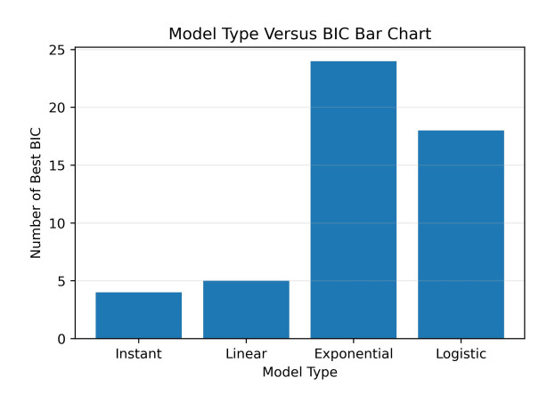
At the onset of the SARS-CoV-2 pandemic in early 2020, only non-pharmaceutical interventions (NPIs) were available to stem the spread of the infection. Much of the early interventions in the US were applied at a state level, with varying levels of strictness and compliance. While NPIs clearly slowed the rate of transmission, it is not clear how these changes are best incorporated into epidemiological models. In order to characterize the effects of early preventative measures, we use a Susceptible-Exposed-Infected-Recovered (SEIR) model and cumulative case counts from US states to analyze the effect of lockdown measures. We test four transition models to simulate the change in transmission rate: instantaneous, linear, exponential, and logarithmic. We find that of the four models examined here, the exponential transition best represents the change in the transmission rate due to implementation of NPIs in the most states, followed by the logistic transition model. The instantaneous and linear models generally lead to poor fits and are the best transition models for the fewest states.
Citation: Gabriel McCarthy, Hana M. Dobrovolny. Determining the best mathematical model for implementation of non-pharmaceutical interventions[J]. Mathematical Biosciences and Engineering, 2025, 22(3): 700-724. doi: 10.3934/mbe.2025026
At the onset of the SARS-CoV-2 pandemic in early 2020, only non-pharmaceutical interventions (NPIs) were available to stem the spread of the infection. Much of the early interventions in the US were applied at a state level, with varying levels of strictness and compliance. While NPIs clearly slowed the rate of transmission, it is not clear how these changes are best incorporated into epidemiological models. In order to characterize the effects of early preventative measures, we use a Susceptible-Exposed-Infected-Recovered (SEIR) model and cumulative case counts from US states to analyze the effect of lockdown measures. We test four transition models to simulate the change in transmission rate: instantaneous, linear, exponential, and logarithmic. We find that of the four models examined here, the exponential transition best represents the change in the transmission rate due to implementation of NPIs in the most states, followed by the logistic transition model. The instantaneous and linear models generally lead to poor fits and are the best transition models for the fewest states.

| [1] |
S. SeyedAlinaghi, P. Mirzapour, O. Dadras, Z. Pashaei, A. Karimi, M. MohsseniPour, et al., Characterization of SARS-CoV-2 different variants and related morbidity and mortality: A systematic review, Eur. J. Med. Res., 26 (2021), 51. https://doi.org/10.1186/s40001-021-00524-8 doi: 10.1186/s40001-021-00524-8

|
| [2] |
N. Chen, M. Zhou, X. Dong, J. Qu, F. Gong, Y. Han, et al., Epidemiological and clinical characteristics of 99 cases of 2019 novel coronavirus pneumonia in Wuhan, China: A descriptive study, Lancet, 395 (2020), 507–513. https://doi.org/10.1016/S0140-6736(20)30211-7 doi: 10.1016/S0140-6736(20)30211-7
|
| [3] |
F. Wu, S. Zhao, B. Yu, Y. M. Chen, W. Wang, Z. G. Song, et al., A new coronavirus associated with human respiratory disease in China, Nature, 579 (2020), 265–271. https://doi.org/10.1038/s41586-020-2008-3 doi: 10.1038/s41586-020-2008-3
|
| [4] |
M. A. Spinelli, D. V. Glidden, E. D. Gennatas, M. Bielecki, C. Beyrer, G. Rutherford, et al., Importance of non-pharmaceutical interventions in lowering the viral inoculum to reduce susceptibility to infection by SARS-CoV-2 and potentially disease severity, Lancet Infect. Dis., 21 (2021), e296–e301. https://doi.org/10.1016/S1473-3099(20)30982-8 doi: 10.1016/S1473-3099(20)30982-8
|
| [5] |
R. F. Rizvi, K. J. T. Craig, R. Hekmat, F. Reyes, B. South, B. Rosario, et al., Effectiveness of non-pharmaceutical interventions related to social distancing on respiratory viral infectious disease outcomes: A rapid evidence-based review and meta-analysis, Sage Open Med., 9. https://doi.org/10.1177/20503121211022973 doi: 10.1177/20503121211022973
|
| [6] |
B. Oppenheim, M. Gallivan, N. K. Madhav, N. Brown, V. Serhiyenko, N. D. Wolfe, et al., Assessing global preparedness for the next pandemic: Development and application of an Epidemic Preparedness Index, BMJ Public Health, 4 (2019), e001157. https://doi.org/10.1136/bmjgh-2018-001157 doi: 10.1136/bmjgh-2018-001157
|
| [7] |
M. N. Miranda, M. Pingarilho, V. Pimentel, A. Torneri, S. G. Seabra, P. J. Libin, et al., A tale of three recent pandemics: Influenza, HIV and SARS-CoV-2, Front. Microbiol., 13 (2022), 889643. https://doi.org/10.3389/fmicb.2022.889643 doi: 10.3389/fmicb.2022.889643
|
| [8] |
K. Seetah, H. Moots, D. Pickel, M. Van Cant, A. Cianciosi, E. Mordecai, et al., Global health needs modernized containment strategies to prepare for the next pandemic, Front. Public Health, 10 (2022), 834451. https://doi.org/10.3389/fpubh.2022.834451 doi: 10.3389/fpubh.2022.834451
|
| [9] |
W. K. Pan, D. Fernandez, S. Tyrovolas, I. Gine-Vazquez, R. R. Dasgupta, B. F. Zaitchik, et al., Heterogeneity in the effectiveness of non-pharmaceutical interventions during the first SARS-CoV2 wave in the United States, Front. Public Health, 9 (2021), 754696. https://doi.org/10.3389/fpubh.2021.754696 doi: 10.3389/fpubh.2021.754696
|
| [10] |
J. L. Guest, C. Del Rio, T. Sanchez, The three steps needed to end the COVID-19 pandemic: Bold public health leadership, rapid innovations, and courageous political will, JMIR Public Health Surveillance, 6 (2020), e19043. https://doi.org/10.2196/19043 doi: 10.2196/19043
|
| [11] |
N. Sharif, K. J. Alzahrani, S. N. Ahmed, R. R. Opu, N. Ahmed, A. Talukder, et al., Protective measures are associated with the reduction of transmission of COVID-19 in bangladesh: A nationwide cross-sectional study, Plos One, 16 (2021), e0260287. https://doi.org/10.1371/journal.pone.0260287 doi: 10.1371/journal.pone.0260287
|
| [12] |
D. Fernandez, I. Gine-Vazquez, M. Morena, A. Koyanagi, M. M. Janko, J. M. Haro, et al., Government interventions and control policies to contain the first COVID-19 outbreak: An analysis of evidence, Scand. J. Public Health, 51 (2023). https://doi.org/10.1177/14034948231156969 doi: 10.1177/14034948231156969
|
| [13] |
M. M. Trivedi, A. Das, Did the timing of state mandated lockdown affect the spread of COVID-19 infection? A county-level ecological study in the united states, J Prev. Med. Public Health, 54 (2021), 238–244. https://doi.org/10.3961/jpmph.21.071 doi: 10.3961/jpmph.21.071
|
| [14] |
P. Zhang, K. Feng, Y. Gong, J. Lee, S. Lomonaco, L. Zhao, Usage of compartmental models in predicting COVID-19 outbreaks, AAPS J., 24 (2022), 98. https://doi.org/10.1208/s12248-022-00743-9 doi: 10.1208/s12248-022-00743-9
|
| [15] |
W. Kermack, A. McKendrick, A contribution to the mathematical theory of epidemics, Proc. R. Soc. London, 115 (1927), 700–721. https://doi.org/10.1098/rspa.1927.0118 doi: 10.1098/rspa.1927.0118
|
| [16] |
N. Perra, Non-pharmaceutical interventions during the COVID-19 pandemic: A review, Phys. Rep., 913 (2021), 1–52. https://doi.org/10.1016/j.physrep.2021.02.001 doi: 10.1016/j.physrep.2021.02.001
|
| [17] |
T. Qiu, H. Xiao, V. Brusic, Estimating the effects of public health measures by SEIR(MH) model of COVID-19 epidemic in local geographic areas, Front. Public Health, 9 (2022), 728525. https://doi.org/10.3389/fpubh.2021.728525 doi: 10.3389/fpubh.2021.728525
|
| [18] |
B. A. van Bunnik, A. L. Morgan, P. R. Bessell, G. Calder-Gerver, F. Zhang, S. Haynes, et al., Segmentation and shielding of the most vulnerable members of the population as elements of an exit strategy from COVID-19 lockdown, Phil. Trans. R. Soc. B, 376 (2021), 20200275. https://doi.org/10.1098/rstb.2020.0275 doi: 10.1098/rstb.2020.0275
|
| [19] |
S. S. Nadim, J. Chattopadhyay, Occurrence of backward bifurcation and prediction of disease transmission with imperfect lockdown: A case study on COVID-19, Chaos Solitons Fractals, 140 (2020), 110163. https://doi.org/10.1016/j.chaos.2020.110163 doi: 10.1016/j.chaos.2020.110163
|
| [20] |
B. Roche, A. Garchitorena, D. Roiz, The impact of lockdown strategies targeting age groups on the burden of COVID-19 in france, Epidemics, 33 (2020), 100424. https://doi.org/10.1016/j.epidem.2020.100424 doi: 10.1016/j.epidem.2020.100424
|
| [21] |
A. Goyal, D. B. Reeves, N. Thakkar, M. Famulare, E. F. Cardozo-Ojeda, B. T. Mayer, et al., Slight reduction in SARS-CoV-2 exposure viral load due to masking results in a significant reduction in transmission with widespread implementation, Sci. Rep., 11 (2021), 11838. https://doi.org/10.1038/s41598-021-91338-5 doi: 10.1038/s41598-021-91338-5
|
| [22] |
C. R. MacIntyre, V. Costantino, A. Chanmugam, The use of face masks during vaccine roll-out in New York City and impact on epidemic control, Vaccine, 39 (2021), 6296–6301. https://doi.org/10.1016/j.vaccine.2021.08.102 doi: 10.1016/j.vaccine.2021.08.102
|
| [23] |
A. Gomes, A. De Cezaro, A model of social distancing for interacting age-distributed multi-populations: An analysis of students' in-person return to schools, Trends Comput. Appl. Math., 23 (2022), 655–671. https://doi.org/10.5540/tcam.2022.023.04.00655 doi: 10.5540/tcam.2022.023.04.00655
|
| [24] |
J. Lee, R. Mendoza, V. Mendoza, J. Lee, Y. Seo, E. Jung, Modelling the effects of social distancing, antiviral therapy, and booster shots on mitigating Omicron spread, Sci. Rep., 13 (2023), 6914. https://doi.org/10.1038/s41598-023-34121-y doi: 10.1038/s41598-023-34121-y
|
| [25] |
L. Matrajt, T. Leung, Evaluating the effectiveness of social distancing interventions to delay or flatten the epidemic curve of coronavirus disease, Emerging Infect. Dis., 26 (2020), 1740–1748. https://doi.org/10.3201/eid2608.201093 doi: 10.3201/eid2608.201093
|
| [26] |
K. P. Vatcheva, J. Sifuentes, T. Oraby, J. C. Maldonado, T. Huber, M. C. Villalobos, Social distancing and testing as optimal strategies against the spread of COVID-19 in the Rio Grande Valley of Texas, Infect. Dis. Modell., 6 (2021), 729–742. https://doi.org/10.1016/j.idm.2021.04.004 doi: 10.1016/j.idm.2021.04.004
|
| [27] |
S. C. Anderson, A. M. Edwards, M. Yerlanov, N. Mulberry, J. E. Stockdale, S. A. Iyaniwura, et al., Quantifying the impact of COVID-19 control measures using a Bayesian model of physical distancing, Plos Genet., 16 (2020), e1008274. https://doi.org/10.1371/journal.pgen.1008274 doi: 10.1371/journal.pgen.1008274
|
| [28] |
T. A. Perkins, G. Espana, Optimal control of the COVID-19 pandemic with non-pharmaceutical interventions, Bull. Math. Biol., 82 (2020), 118. https://doi.org/10.1007/s11538-020-00795-y doi: 10.1007/s11538-020-00795-y
|
| [29] |
C. Mondal, D. Adak, A. Majumder, N. Bairagi, Mitigating the transmission of infection and death due to SARS-CoV-2 through non-pharmaceutical interventions and repurposing drugs, ISA Trans., 124 (2022), 236–246. https://doi.org/10.1016/j.isatra.2020.09.015 doi: 10.1016/j.isatra.2020.09.015
|
| [30] |
S. Hsiang, D. Allen, S. Annan-Phan, K. Bell, I. Bolliger, T. Chong, et al., The effect of large-scale anti-contagion policies on the COVID-19 pandemic, Nature, 584 (2020), 262–267. https://doi.org/10.1038/s41586-020-2404-8 doi: 10.1038/s41586-020-2404-8
|
| [31] |
M. A. Acuña-Zegarra, M. Santana-Cibrian, J. X. Velasco-Hernandez, Modeling behavioral change and COVID-19 containment in Mexico: A trade-off between lockdown and compliance, Math. Biosci., 325 (2020), 108370. https://doi.org/10.1016/j.mbs.2020.108370 doi: 10.1016/j.mbs.2020.108370
|
| [32] |
M. L. Childs, M. P. Kain, M. J. Harris, D. Kirk, L. Couper, N. Nova, et al., The impact of long-term non-pharmaceutical interventions on COVID-19 epidemic dynamics and control: The value and limitations of early models, Proc. R. Soc. B, 288 (2021), 20210811. https://doi.org/10.1098/rspb.2021.0811 doi: 10.1098/rspb.2021.0811
|
| [33] |
C. N. Ngonghala, E. Iboi, S. Eikenberry, M. Scotch, C. R. MacIntyre, M. H. Bonds, et al., Mathematical assessment of the impact of non-pharmaceutical interventions on curtailing the 2019 novel coronavirus, Math. Biosci., 325 (2020), 108364. https://doi.org/10.1016/j.mbs.2020.108364 doi: 10.1016/j.mbs.2020.108364
|
| [34] |
S. Fuderer, C. Kuttler, M. Hoelscher, L. C. Hinske, N. Castelletti, Data suggested hospitalization as critical indicator of the severity of the COVID-19 pandemic, even at its early stages, Math. Biosci. Eng., 20 (2023), 10304–10338. https://doi.org/10.3934/mbe.2023452 doi: 10.3934/mbe.2023452
|
| [35] |
L. Tarrataca, C. M. Dias, D. B. Haddad, E. F. De Arruda, Flattening the curves: On-off lock-down strategies for COVID-19 with an application to Brazil, J. Math. Ind., 11 (2021), 2. https://doi.org/10.1186/s13362-020-00098-w doi: 10.1186/s13362-020-00098-w
|
| [36] |
M. V. Barbarossa, J. Fuhrmann, J. H. Meinke, S. Krieg, H. V. Varma, N. Castelletti, et al., Modeling the spread of COVID-19 in germany: Early assessment and possible scenarios, Plos One, 15 (2020), e0238559. https://doi.org/10.1371/journal.pone.0238559 doi: 10.1371/journal.pone.0238559
|
| [37] |
S. Lai, N. W. Ruktanonchai, L. Zhou, O. Prosper, W. Luo, J. R. Floyd, et al., Effect of non-pharmaceutical interventions to contain COVID-19 in China, Nature, 585 (2020), 410–413. https://doi.org/10.1038/s41586-020-2293-x doi: 10.1038/s41586-020-2293-x
|
| [38] |
K. D. Min, H. Kang, J. Y. Lee, S. Jeon, S. il Cho, Estimating the effectiveness of non-pharmaceutical interventions on COVID-19 control in Korea, J. Korean Med. Sci., 35 (2020), 1146164. https://doi.org/10.3346/jkms.2020.35.e321 doi: 10.3346/jkms.2020.35.e321
|
| [39] |
N. G. Davies, A. J. Kucharski, R. M. Eggo, A. Gimma, W. J. Edmunds, T. Jombart, et al., Effects of non-pharmaceutical interventions on COVID-19 cases, deaths, and demand for hospital services in the UK: A modelling study, Lancet Public Health, 5 (2020), e375–e385. https://doi.org/10.1016/S2468-2667(20)30133-X doi: 10.1016/S2468-2667(20)30133-X
|
| [40] |
K. van Zandvoort, C. I. Jarvis, C. A. B. Pearson, N. G. Davies, CMMID COVID-19 working group, R. Ratnayake, et al., Response strategies for COVID-19 epidemics in African settings: A mathematical modelling study, BMC Med., 18 (2020), 324. https://doi.org/10.1186/s12916-020-01789-2 doi: 10.1186/s12916-020-01789-2
|
| [41] |
A. de Visscher, The COVID-19 pandemic: Model-based evaluation of non-pharmaceutical interventions and prognoses, Nonlinear Dyn., 101 (2020), 1871–1887. https://doi.org/10.1007/s11071-020-05861-7 doi: 10.1007/s11071-020-05861-7
|
| [42] |
G. C. Calafiore, C. Novara, C. Possieri, A time-varying SIRD model for the COVID-19 contagion in Italy, Annu. Rev. Control, 50 (2020), 361–372. https://doi.org/10.1016/j.arcontrol.2020.10.005 doi: 10.1016/j.arcontrol.2020.10.005
|
| [43] |
M. Kantner, T. Koprucki, Beyond just "flattening the curve": Optimal control of epidemics with purely non-pharmaceutical interventions, J. Math. Ind., 10 (2020), 23. https://doi.org/10.1186/s13362-020-00091-3 doi: 10.1186/s13362-020-00091-3
|
| [44] |
S. Kim, Y. Ko, Y. J. Kim, E. Jung, The impact of social distancing and public behavior changes on COVID-19 transmission dynamics in the Republic of Korea, Plos One, 15 (2020), e0238684. https://doi.org/10.1371/journal.pone.0238684 doi: 10.1371/journal.pone.0238684
|
| [45] |
S. E. Eikenberry, M. Mancuso, E. Iboi, T. Phan, K. Eikenberry, Y. Kuang, et al., To mask or not to mask: Modeling the potential for face mask use by the general public to curtail the COVID-19 pandemic, Infect. Dis. Modell., 5 (2020), 293–308. https://doi.org/10.1016/j.idm.2020.04.001 doi: 10.1016/j.idm.2020.04.001
|
| [46] |
T. Bai, D. Wang, W. Dai, A modified SEIR model with a jump in the transmission parameter applied to COVID-19 data on Wuhan, Stat, 11 (2022), e511. https://doi.org/10.1002/sta4.511 doi: 10.1002/sta4.511
|
| [47] |
H. Xin, Y. Li, P. Wu, Z. Li, E. H. Y. Lau, Y. Qin, et al., Estimating the latent period of coronavirus disease 2019 (COVID-19), Clin. Infect. Dis., 74 (2021), 1678–1681, https://doi.org/10.1093/cid/ciab746 doi: 10.1093/cid/ciab746
|
| [48] | CDC, Ending isolation and precautions for people with COVID-19: Interim guidance. Available from: https://www.cdc.gov/coronavirus/2019-ncov/hcp/duration-isolation.html. |
| [49] | CDC, Clinical presentation. Available from: https://www.cdc.gov/coronavirus/2019-ncov/hcp/clinical-care/clinical-considerations-presentation.html. |
| [50] |
C. Turkun, M. Golgeli, F. M. Atay, A mathematical interpretation for outbreaks of bacterial meningitis under the effect of time-dependent transmission parameters, Nonlinear Dyn., 111 (2023), 14467–14484. https://doi.org/10.1007/s11071-023-08577-6 doi: 10.1007/s11071-023-08577-6
|
| [51] |
X. Y. Zhao, S. M. Guo, M. Ghosh, X. Z. Li, Stability and persistence of an avian influenza epidemic model with impacts of climate change, Discrete Dyn. Nat. Soc., 2016 (2016). https://doi.org/10.1155/2016/7871251 doi: 10.1155/2016/7871251
|
| [52] |
S. Zhang, Y. Zhao, Estimating and comparing case fatality rates of pandemic influenza A (H1N1) 2009 in its early stage in different countries, J. Public Health, 20 (2012), 607–613. https://doi.org/10.1007/s10389-012-0498-7 doi: 10.1007/s10389-012-0498-7
|
| [53] |
J. P. Mateus, C. M. Silva, Existence of periodic solutions of a periodic seirs model with general incidence, Nonlinear Anal. Real World Appl., 34 (2017), 379–402. https://doi.org/10.1016/j.nonrwa.2016.09.013 doi: 10.1016/j.nonrwa.2016.09.013
|
| [54] |
P. E. Kloeden, C. Poetzsche, Nonautonomous bifurcation scenarios in sir models, Math. Methods Appl. Sci., 38 (2015), 3495–3518. https://doi.org/10.1002/mma.3433 doi: 10.1002/mma.3433
|
| [55] |
J. Liu, T. Zhang, Analysis of a nonautonomous epidemic model with density dependent birth rate, Appl. Math. Modell., 34 (2010), 866–877. https://doi.org/10.1016/j.apm.2009.07.004 doi: 10.1016/j.apm.2009.07.004
|
| [56] | B. Efron, R. Tibshirani, Bootstrap methods for standard errors, confidence intervals, and other measures of statistical accuracy, Stat. Sci., 1 (1986), 54–75. |
| [57] |
P. Stoica, Y. Selen, Model-order selection, IEEE Signal Process. Mag., 21 (2004), 36–47. https://doi.org/10.1109/MSP.2004.1311138 doi: 10.1109/MSP.2004.1311138
|
| [58] |
J. Noh, G. Danuser, Estimation of the fraction of COVID-19 infected people in us states and countries worldwide, Plos One, 16 (2021). https://doi.org/10.1371/journal.pone.0246772 doi: 10.1371/journal.pone.0246772
|
| [59] |
E. R. White, L. Hebert-Dufresne, State-level variation of initial COVID-19 dynamics in the United States, Plos One, 15. https://doi.org/10.1371/journal.pone.0240648 doi: 10.1371/journal.pone.0240648
|
| [60] |
H. M. Dobrovolny, Modeling the role of asymptomatics in infection spread with application to SARS-CoV-2, Plos One, 15 (2020), e0236976. https://doi.org/10.1371/journal.pone.0236976 doi: 10.1371/journal.pone.0236976
|
| [61] |
C. D. Guss, L. Boyd, K. Perniciaro, D. C. Free, J. R. Free, M. T. Tuason, The politics of COVID-19: Differences between U.S. red and blue states in COVID-19 regulations and deaths, Health Policy Open, 5 (2023), 100107. https://doi.org/10.1016/j.hpopen.2023.100107 doi: 10.1016/j.hpopen.2023.100107
|
| [62] |
I. W. Nader, E. L. Zeilinger, D. Jomar, C. Zauchner, Onset of effects of non-pharmaceutical interventions on COVID-19 infection rates in 176 countries, BMC Public Health, 21 (2021), 1472. https://doi.org/10.1186/s12889-021-11530-0 doi: 10.1186/s12889-021-11530-0
|
| [63] |
R. Nistal, M. de la Sen, J. Gabirondo, S. Alonso-Quesada, A. J. Garrido, I. Garrido, A modelization of the propagation of COVID-19 in regions of Spain and Italy with evaluation of the transmission rates related to the intervention measures, Biology, 10 (2021), 121. https://doi.org/10.3390/biology10020121 doi: 10.3390/biology10020121
|
| [64] |
V. Tselios, The timing of implementation of COVID-19 lockdown policies: Does decentralization matter, Publius J. Federalism, 54 (2024), 34–58. https://doi.org/10.1093/publius/pjad021 doi: 10.1093/publius/pjad021
|
| [65] |
J. E. Harris, Timely epidemic monitoring in the presence of reporting delays: Anticipating the COVID-19 surge in New York City, September 2020, BMC Public Health, 22 (2022), 871. https://doi.org/10.1186/s12889-022-13286-7 doi: 10.1186/s12889-022-13286-7
|
| [66] |
S. A. Iyaniwura, M. Rabiu, J. F. David, J. D. Kong, Assessing the impact of adherence to non-pharmaceutical interventions and indirect transmission on the dynamics of COVID-19: A mathematical modelling study, Math. Biosci. Eng., 18 (2021), 8905–8932. https://doi.org/10.3934/mbe.2021439 doi: 10.3934/mbe.2021439
|
| [67] |
J. P. N. N'konzi, C. W. Chukwu, F. Nyabadza, Effect of time-varying adherence to non-pharmaceutical interventions on the occurrence of multiple epidemic waves: A modeling study, Front. Public Health, 10 (2022), 1087683. https://doi.org/10.3389/fpubh.2022.1087683 doi: 10.3389/fpubh.2022.1087683
|
| [68] |
J. Dehning, J. Zierenberg, F. P. Spitzner, M. Wibral, J. P. Neto, M. Wilczek, et al., Inferring change points in the spread of COVID-19 reveals the effectiveness of interventions, Science, 369 (2020), eabb9789. https://doi.org/10.1126/science.abb9789 doi: 10.1126/science.abb9789
|
| [69] |
L. O. Náraigh, Á. Byrne, Piecewise-constant optimal control strategies for controlling the outbreak of COVID-19 in the Irish population, Math. Biosci., 330 (2020), 108496. https://doi.org/10.1016/j.mbs.2020.108496 doi: 10.1016/j.mbs.2020.108496
|
| [70] |
R. Alisic, P. E. Pare, H. Sandberg, Change time estimation uncertainty in nonlinear dynamical systems with applications to COVID-19, Int. J. Robust Nonlinear Control, 33 (2023), 4732–4760. https://doi.org/10.1002/rnc.5974 doi: 10.1002/rnc.5974
|
| [71] |
A. Vallee, Heterogeneity of the COVID-19 pandemic in the United States of America: A geo-epidemiological perspective, Front. Public Health, 19 (2022), 818989. https://doi.org/10.3389/fpubh.2022.818989 doi: 10.3389/fpubh.2022.818989
|
| [72] |
L. J. Thomas, P. Huang, F. Yin, X. I. Luo, Z. W. Almquist, J. R. Hipp, et al., Spatial heterogeneity can lead to substantial local variations in COVID-19 timing and severity, Proc. Natl. Acad. Sci. U.S.A., 117 (2020), 24180–24187. https://doi.org/10.1073/pnas.2011656117 doi: 10.1073/pnas.2011656117
|
| [73] |
V. A. Karatayev, M. Anand, C. T. Bauch, Local lockdowns outperform global lockdown on the far side of the COVID-19 epidemic curve, Proc. Natl. Acad. Sci. U.S.A., 117 (2020), 24575–24580. https://doi.org/10.1073/pnas.2014385117 doi: 10.1073/pnas.2014385117
|
| [74] |
E. Armstrong, M. Runge, J. Gerardin, Identifying the measurements required to estimate rates of COVID-19 transmission, infection, and detection, using variational data assimilation, Infect. Dis. Modell., 6 (2021), 133–147. https://doi.org/10.1016/j.idm.2020.10.010 doi: 10.1016/j.idm.2020.10.010
|
| [75] |
S. Chowdhury, M. Forkan, P. Agarwal, S. Muyeen, S. F. Ahmad, A. S. Ali, Modeling the SARS-CoV-2 parallel transmission dynamics: Asymptomatic and symptomatic pathways, Comput. Biol. Med., 143 (2022), 105264. https://doi.org/10.1016/j.compbiomed.2022.105264 doi: 10.1016/j.compbiomed.2022.105264
|
| [76] |
A. Mishra, S. Purohit, K. Owolabi, Y. Sharma, A nonlinear epidemiological model considering asymptotic and quarantine classes for SARS CoV-2 virus, Chaos Solitons Fractals, 138 (2020), 109953. https://doi.org/10.1016/j.chaos.2020.109953 doi: 10.1016/j.chaos.2020.109953
|
| [77] |
L. X. Feng, S. L. Jing, S. K. Hu, D. F. Wang, H. F. Huo, Modelling the effects of media coverage and quarantine on the COVID-19 infections in the UK, Math. Biosci. Eng., 17 (2020), 3618–3636. https://doi.org/10.3934/mbe.2020204 doi: 10.3934/mbe.2020204
|
| [78] |
B. Ivorra, M. Ferrandez, M. Vela-Perez, A. Ramos, Mathematical modeling of the spread of the coronavirus disease 2019 (COVID-19) taking into account the undetected infections. the case of China, Commun. Nonlinear Sci. Numer. Simul., 88 (2022), 105303. https://doi.org/10.1016/j.cnsns.2020.105303 doi: 10.1016/j.cnsns.2020.105303
|
| [79] |
A. M. Salman, I. Ahmed, M. H. Mohd, M. S. Jamiluddin, M. A. Dheyab, Scenario analysis of COVID-19 transmission dynamics in Malaysia with the possibility of reinfection and limited medical resources scenarios, Comput. Biol. Med., 133 (2021), 104372. https://doi.org/10.1016/j.compbiomed.2021.104372 doi: 10.1016/j.compbiomed.2021.104372
|
| [80] |
B. Shayak, M. M. Sharma, M. Gaur, A. K. Mishra, Impact of reproduction number on the multiwave spreading dynamics of COVID-19 with temporary immunity: A mathematical model, Int. J. Infect. Dis., 104 (2021), 649–654. https://doi.org/10.1016/j.ijid.2021.01.018 doi: 10.1016/j.ijid.2021.01.018
|
| [81] |
G. Gonzalez-Parra, M. Diaz-Rodriguez, A. J. Arenas, Mathematical modeling to study the impact of immigration on the dynamics of the COVID-19 pandemic: A case study for Venezuela, Spatial Spatio-temporal Epidemiol., 43 (2022), 100532. https://doi.org/10.1016/j.sste.2022.100532 doi: 10.1016/j.sste.2022.100532
|
| [82] |
D. De Ridder, J. Sandoval, N. Vuilleumier, A. S. Azman, S. Stringhini, L. Kaiser, et al., Socioeconomically disadvantaged neighborhoods face increased persistence of SARS-CoV-2 clusters, Front. Public Health, 8 (2021), 626090. https://doi.org/10.3389/fpubh.2020.626090 doi: 10.3389/fpubh.2020.626090
|
| [83] |
K. T. L. Sy, L. F. White, B. E. Nichols, Population density and basic reproductive number of COVID-19 across United States counties, Plos One, 16 (2021), e0249271. https://doi.org/10.1371/journal.pone.0249271 doi: 10.1371/journal.pone.0249271
|
| [84] |
A. James, M. Plank, R. Binny, A. Lustig, K. Hannah, S. Hendy, et al., A structured model for COVID-19 spread: Modelling age and healthcare inequities, Math. Med. Biol., 38 (2021), 299–313. https://doi.org/10.1093/imammb/dqab006 doi: 10.1093/imammb/dqab006
|
| [85] |
Y. Wu, T. A. Mooring, M. Linz, Policy and weather influences on mobility during the early US COVID-19 pandemic, Proc. Natl. Acad. Sci. U.S.A., 118 (2021), e2018185118. https://doi.org/10.1073/pnas.2018185118 doi: 10.1073/pnas.2018185118
|

Figures(9) / Tables(2)

Gabriel McCarthy, Hana M. Dobrovolny. Determining the best mathematical model for implementation of non-pharmaceutical interventions[J]. Mathematical Biosciences and Engineering, 2025, 22(3): 700-724. doi: 10.3934/mbe.2025026


 DownLoad: