Cross-modal missing time-series imputation using dense spatio-temporal transformer nets

Xusheng Qian; Teng Zhang; Meng Miao; Gaojun Xu; Xuancheng Zhang; Wenwu Yu; Duxin Chen; Xusheng Qian; Teng Zhang; Meng Miao; Gaojun Xu; Xuancheng Zhang; Wenwu Yu; Duxin Chen

doi:10.3934/mbe.2024220

Mathematical Biosciences and Engineering

2024, Volume 21, Issue 4: 4989-5006. doi: 10.3934/mbe.2024220

Previous Article Next Article

Research article Special Issues

Cross-modal missing time-series imputation using dense spatio-temporal transformer nets

1.
State Grid Jiangsu Electric Power Company Limited Marketing Service Center, Nanjing 210019, China
2.
Jiangsu Key Laboratory of Networked Collective Intelligence, School of Mathematics, Southeast University, Nanjing 211189, China

Academic Editor: Xiaodi Li

Received: 06 November 2023 Revised: 20 January 2024 Accepted: 24 January 2024 Published: 01 March 2024

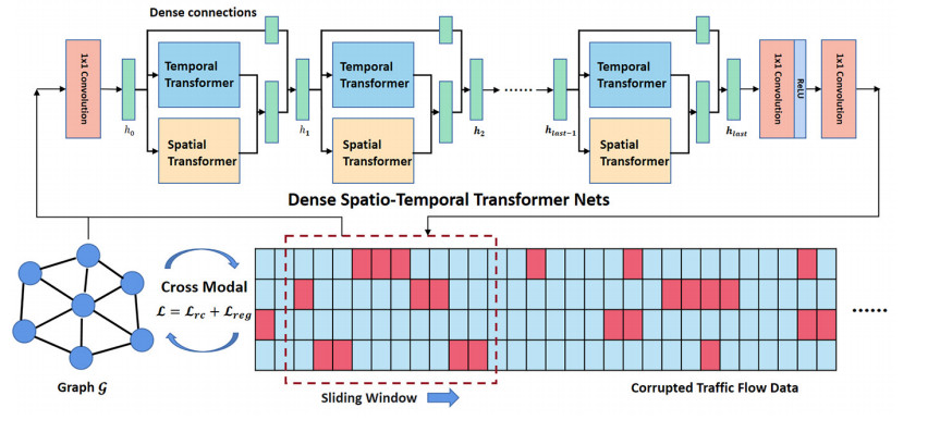
Due to irregular sampling or device failure, the data collected from sensor network has missing value, that is, missing time-series data occurs. To address this issue, many methods have been proposed to impute random or non-random missing data. However, the imputation accuracy of these methods are not accurate enough to be applied, especially in the case of complete data missing (CDM). Thus, we propose a cross-modal method to impute time-series missing data by dense spatio-temporal transformer nets (DSTTN). This model embeds spatial modal data into time-series data by stacked spatio-temporal transformer blocks and deployment of dense connections. It adopts cross-modal constraints, a graph Laplacian regularization term, to optimize model parameters. When the model is trained, it recovers missing data finally by an end-to-end imputation pipeline. Various baseline models are compared by sufficient experiments. Based on the experimental results, it is verified that DSTTN achieves state-of-the-art imputation performance in the cases of random and non-random missing. Especially, the proposed method provides a new solution to the CDM problem.
- time-series data missing,
- complete data missing,
- time-series data imputation,
- cross-modal data fusion,
- dense spatio-temporal transformer nets
Citation: Xusheng Qian, Teng Zhang, Meng Miao, Gaojun Xu, Xuancheng Zhang, Wenwu Yu, Duxin Chen. Cross-modal missing time-series imputation using dense spatio-temporal transformer nets[J]. Mathematical Biosciences and Engineering, 2024, 21(4): 4989-5006. doi: 10.3934/mbe.2024220

Related Papers:

Abstract

Due to irregular sampling or device failure, the data collected from sensor network has missing value, that is, missing time-series data occurs. To address this issue, many methods have been proposed to impute random or non-random missing data. However, the imputation accuracy of these methods are not accurate enough to be applied, especially in the case of complete data missing (CDM). Thus, we propose a cross-modal method to impute time-series missing data by dense spatio-temporal transformer nets (DSTTN). This model embeds spatial modal data into time-series data by stacked spatio-temporal transformer blocks and deployment of dense connections. It adopts cross-modal constraints, a graph Laplacian regularization term, to optimize model parameters. When the model is trained, it recovers missing data finally by an end-to-end imputation pipeline. Various baseline models are compared by sufficient experiments. Based on the experimental results, it is verified that DSTTN achieves state-of-the-art imputation performance in the cases of random and non-random missing. Especially, the proposed method provides a new solution to the CDM problem.

References

[1]	X. Li, X. Yang, J. Cao, Event-triggered impulsive control for nonlinear delay systems, Automatica, 117 (2020), 108981. https://doi.org/10.1016/j.automatica.2020.108981 doi: 10.1016/j.automatica.2020.108981
[2]	X. Li, D. Peng, J. Cao, Lyapunov stability for impulsive systems via event-triggered impulsive control, IEEE Trans. Autom. Control, 65 (2020), 4908–4913. https://doi.org/10.1109/TAC.2020.2964558 doi: 10.1109/TAC.2020.2964558
[3]	P. Dai, W. Yu, G. Wen, S. Baldi, Distributed reinforcement learning algorithm for dynamic economic dispatch with unknown generation cost functions, IEEE Trans. Ind. Inf., 16 (2019), 2258–2267. https://doi.org/10.1109/TII.2019.2933443 doi: 10.1109/TII.2019.2933443
[4]	X. Miao, Y. Wu, L. Chen, Y. Gao, J. Wang, J. Yin, Efficient and effective data imputation with influence functions, in Proceedings of the VLDB Endowment, 15 (2021), 624–632. https://doi.org/10.14778/3494124.3494143
[5]	A. Blázquez-García, K. Wickstrøm, S. Yu, K. Ø. Mikalsen, A. Boubekki, A. Conde, et al., Selective imputation for multivariate time series datasets with missing values, IEEE Trans. Knowl. Data Eng., 2023 (2023). https://doi.org/10.1109/TKDE.2023.3240858 doi: 10.1109/TKDE.2023.3240858
[6]	Y. Li, Z. Li, L. Li, Missing traffic data: comparison of imputation methods, IET Intell. Transp. Syst., 8 (2014), 51–57. https://doi.org/10.1049/iet-its.2013.0052 doi: 10.1049/iet-its.2013.0052
[7]	C. Zhang, Y. Cui, Z. Han, J. T. Zhou, H. Fu, Q. Hu, Deep partial multi-view learning, IEEE Trans. Pattern Anal. Mach. Intell., 44 (2020), 2402–2415. https://doi.org/10.1109/TPAMI.2020.3037734 doi: 10.1109/TPAMI.2020.3037734
[8]	M. Yang, Y. Li, P. Hu, J. Bai, J. C. Lv, X. Peng, Robust multi-view clustering with incomplete information, IEEE Trans. Pattern Anal. Mach. Intell., 45 (2022), 1055–1069. https://doi.org/10.1109/TPAMI.2022.3155499 doi: 10.1109/TPAMI.2022.3155499
[9]	X. Miao, Y. Wu, L. Chen, Y. Gao, J. Yin, An experimental survey of missing data imputation algorithms, IEEE Trans. Knowl. Data Eng., 2022 (2022). https://doi.org/10.1109/TKDE.2022.3186498 doi: 10.1109/TKDE.2022.3186498
[10]	M. Kang, R. Zhu, D. Chen, X. Liu, W. Yu, CM-GAN: A cross-modal generative adversarial network for imputing completely missing data in digital industry, IEEE Trans. Neural Networks Learn. Syst., 2023 (2023). https://doi.org/10.1109/TNNLS.2023.3284666 doi: 10.1109/TNNLS.2023.3284666
[11]	J. Wang, C. Lan, C. Liu, Y. Ouyang, T. Qin, W. Lu, et al., Generalizing to unseen domains: A survey on domain generalization, IEEE Trans. Knowl. Data Eng., 2022 (2022). https://doi.org/10.24963/ijcai.2021/628 doi: 10.24963/ijcai.2021/628
[12]	B. Sun, L. Ma, W. Cheng, W. Wen, P. Goswami, G. Bai, An improved k-nearest neighbours method for traffic time series imputation, in 2017 Chinese Automation Congress, (2017), 7346–7351. https://doi.org/10.1109/CAC.2017.8244105
[13]	X. Chen, Z. He, L. Sun, A bayesian tensor decomposition approach for spatiotemporal traffic data imputation, Transp. Res. Part C Emerging Technol., 98 (2019), 73–84. https://doi.org/10.1016/j.trc.2018.11.003 doi: 10.1016/j.trc.2018.11.003
[14]	S. Coogan, C. Flores, P. Varaiya, Traffic predictive control from low-rank structure, Transp. Res. Part B Methodol., 97 (2017), 1–22. https://doi.org/10.1016/j.trb.2016.11.013 doi: 10.1016/j.trb.2016.11.013
[15]	H. Tan, G. Feng, J. Feng, W. Wang, Y. J. Zhang, F. Li, A tensor-based method for missing traffic data completion, Transp. Res. Part C Emerging Technol., 28 (2013), 15–27. https://doi.org/10.1016/j.trc.2012.12.007 doi: 10.1016/j.trc.2012.12.007
[16]	X. Chen, M. Lei, N. Saunier, L. Sun, Low-rank autoregressive tensor completion for spatiotemporal traffic data imputation, IEEE Trans. Intell. Transp. Syst., 23 (2022), 12301–12310. https://doi.org/10.1109/TITS.2021.3113608 doi: 10.1109/TITS.2021.3113608
[17]	Y. Duan, Y. Lv, Y. L. Liu, F. Y. Wang, An efficient realization of deep learning for traffic data imputation, Transp. Res. Part C Emerging Technol., 72 (2016), 168–181. https://doi.org/10.1016/j.trc.2016.09.015 doi: 10.1016/j.trc.2016.09.015
[18]	Y. Tian, K. Zhang, J. Li, X. Lin, B. Yang, LSTM-based traffic flow prediction with missing data, Neurocomputing, 318 (2018), 297–305. https://doi.org/10.1016/j.neucom.2018.08.067 doi: 10.1016/j.neucom.2018.08.067
[19]	Y. Chen, Y. Lv, F. Y. Wang, Traffic flow imputation using parallel data and generative adversarial networks, IEEE Trans. Intell. Transp. Syst., 21 (2019), 1624–1630. https://doi.org/10.1109/TITS.2019.2910295 doi: 10.1109/TITS.2019.2910295
[20]	X. Miao, Y. Wu, J. Wang, Y. Gao, X. Mao, J. Yin, Generative semi-supervised learning for multivariate time series imputation, in Proceedings of the AAAI conference on artificial intelligence, 35 (2021), 8983–8991. https://doi.org/10.1609/aaai.v35i10.17086
[21]	Y. Yao, B. Gu, Z. Su, M. Guizani, MVSTGN: A multi-view spatial-temporal graph network for cellular traffic prediction, IEEE Trans. Mobile Comput., 2021 (2021). https://doi.org/10.1109/TMC.2021.3129796 doi: 10.1109/TMC.2021.3129796
[22]	T. Baltrušaitis, C. Ahuja, L. P. Morency, Multimodal machine learning: A survey and taxonomy, IEEE Trans. Pattern Anal. Mach. Intell., 41 (2018), 423–443. https://doi.org/10.1109/TPAMI.2018.2798607 doi: 10.1109/TPAMI.2018.2798607
[23]	D. Wang, Y. Yan, R. Qiu, Y. Zhu, K. Guan, A. Margenot, et al., Networked time series imputation via position-aware graph enhanced variational autoencoders, in Proceedings of the 29th ACM SIGKDD Conference on Knowledge Discovery and Data Mining, (2023), 2256–2268. https://doi.org/10.1145/3580305.3599444
[24]	D. Chen, Q. Shao, Z. Liu, W. Yu, C. L. P. Chen, Ridesourcing behavior analysis and prediction: A network perspective, IEEE Trans. Intell. Transp. Syst., 23 (2022), 1274–1283. https://doi.org/10.1109/TITS.2020.3023951 doi: 10.1109/TITS.2020.3023951
[25]	S. Lee, D. B. Fambro, Application of subset autoregressive integrated moving average model for short-term freeway traffic volume forecasting, Transp. Res. Record, 1678 (1999), 179–188. https://doi.org/10.3141/1678-22 doi: 10.3141/1678-22
[26]	M. Zhong, S. Sharma, P. Lingras, Genetically designed models for accurate imputation of missing traffic counts, Transp. Res. Record, 1879 (2004), 71–79. https://doi.org/10.3141/1879-09 doi: 10.3141/1879-09
[27]	L. Qu, L. Li, Y. Zhang, J. Hu, PPCA-based missing data imputation for traffic flow volume: A systematical approach, IEEE Trans. Intell. Transp. Syst., 10 (2009), 512–522. https://doi.org/10.1109/TITS.2009.2026312 doi: 10.1109/TITS.2009.2026312
[28]	L. Li, Y. Li, Z. Li, Efficient missing data imputing for traffic flow by considering temporal and spatial dependence, Transp. Res. Part C Emerging Technol., 34 (2013), 108–120. https://doi.org/10.1016/j.trc.2013.05.008 doi: 10.1016/j.trc.2013.05.008
[29]	J. Tang, G. Zhang, Y. Wang, H. Wang, F. Liu, A hybrid approach to integrate fuzzy c-means based imputation method with genetic algorithm for missing traffic volume data estimation, Transp. Res. Part C Emerging Technol., 51 (2015), 29–40. https://doi.org/10.1016/j.trc.2014.11.003 doi: 10.1016/j.trc.2014.11.003
[30]	S. Wang, G. Mao, Missing data estimation for traffic volume by searching an optimum closed cut in urban networks, IEEE Trans. Intell. Transp. Syst., 20 (2018), 75–86. https://doi.org/10.1109/TITS.2018.2801808 doi: 10.1109/TITS.2018.2801808
[31]	Y. Wang, Y. Zhang, X. Piao, H. Liu, K. Zhang, Traffic data reconstruction via adaptive spatial-temporal correlations, IEEE Trans. Intell. Transp. Syst., 20 (2018), 1531–1543. https://doi.org/10.1109/TITS.2018.2854968 doi: 10.1109/TITS.2018.2854968
[32]	X. Chen, Z. He, J. Wang, Spatial-temporal traffic speed patterns discovery and incomplete data recovery via svd-combined tensor decomposition, Transp. Res. Part C Emerging Technol., 86 (2018), 59–77. https://doi.org/10.1016/j.trc.2017.10.023 doi: 10.1016/j.trc.2017.10.023
[33]	Z. Cui, R. Ke, Z. Pu, Y. Wang, Stacked bidirectional and unidirectional lstm recurrent neural network for forecasting network-wide traffic state with missing values, Transp. Res. Part C Emerging Technol., 118 (2020), 102674. https://doi.org/10.1016/j.trc.2020.102674 doi: 10.1016/j.trc.2020.102674
[34]	X. Kong, W. Zhou, G. Shen, W. Zhang, N. Liu, Y. Yang, Dynamic graph convolutional recurrent imputation network for spatiotemporal traffic missing data, Knowl. Based Syst., 261 (2023), 110188. https://doi.org/10.1016/j.knosys.2022.110188 doi: 10.1016/j.knosys.2022.110188
[35]	G. Shen, W. Zhou, W. Zhang, N. Liu, Z. Liu, X. Kong, Bidirectional spatial–temporal traffic data imputation via graph attention recurrent neural network, Neurocomputing, 531 (2023), 151–162. https://doi.org/10.1016/j.neucom.2023.02.017 doi: 10.1016/j.neucom.2023.02.017
[36]	W. Zhang, P. Zhang, Y. Yu, X. Li, S. A. Biancardo, J. Zhang, Missing data repairs for traffic flow with self-attention generative adversarial imputation net, IEEE Trans. Intell. Transp. Syst., 23 (2021), 7919–7930. https://doi.org/10.1109/TITS.2021.3074564 doi: 10.1109/TITS.2021.3074564
[37]	M. Kang, R. Zhu, D. Chen, C. Li, W. Gu, X. Qian, et al., A cross-modal generative adversarial network for scenarios generation of renewable energy, IEEE Trans. Power Syst., 2023 (2023). https://doi.org/10.1109/TPWRS.2023.3277698 doi: 10.1109/TPWRS.2023.3277698
[38]	L. Li, J. Zhang, Y. Wang, B. Ran, Missing value imputation for traffic-related time series data based on a multi-view learning method, IEEE Trans. Intell. Transp. Syst., 20 (2018), 2933–2943. https://doi.org/10.1109/TITS.2018.2869768 doi: 10.1109/TITS.2018.2869768
[39]	A. Vaswani, N. Shazeer, N. Parmar, J. Uszkoreit, L. Jones, A. N. Gomez, et al., Attention is all you need, in Advances in Neural Information Processing Systems, (2017), 5998–6008.
[40]	D. P. Kingma, J. Ba, ADAM: A method for stochastic optimization, in International Conference on Learning Representations, 2015.
[41]	Z. Cui, K. Henrickson, R. Ke, Y. Wang, Traffic graph convolutional recurrent neural network: A deep learning framework for network-scale traffic learning and forecasting, IEEE Trans. Intell. Transp. Syst., 21 (2019), 4883–4894. https://doi.org/10.1109/TITS.2019.2950416 doi: 10.1109/TITS.2019.2950416
[42]	M. Arjovsky, S. Chintala, L. Bottou, Wasserstein generative adversarial networks, in International Conference on Machine Learning, (2017), 214–223.

Reader Comments

Your name:*

Email:*
© 2024 the Author(s), licensee AIMS Press. This is an open access article distributed under the terms of the Creative Commons Attribution License (http://creativecommons.org/licenses/by/4.0)