Impact of general incidence function on three-strain SEIAR model

Manoj Kumar Singh; Anjali.; Brajesh K. Singh; Carlo Cattani; Manoj Kumar Singh; Anjali.; Brajesh K. Singh; Carlo Cattani

doi:10.3934/mbe.2023873

Mathematical Biosciences and Engineering

2023, Volume 20, Issue 11: 19710-19731. doi: 10.3934/mbe.2023873

Previous Article Next Article

Research article Special Issues

Impact of general incidence function on three-strain SEIAR model

1.
Faculty of Mathematics & Computing, Department of Mathematics & Statistics, Banasthali Vidyapith, Rajasthan 304022, India
2.
Department of Mathematics, Babasaheb Bhimrao Ambedkar University, Lucknow 226025, India
3.
Department of Mathematics and Informatics, Azerbaijan University, J. Hajibeyli str., AZ1007, Baku
4.
Azerbaijan Engineering School, DEIM, University of Tuscia, P.le dellUniversità, Viterbo 01100, Italy

Academic Editor: Yang Kuang

Received: 11 June 2023 Revised: 26 September 2023 Accepted: 27 September 2023 Published: 26 October 2023

We investigate the behavior of a complex three-strain model with a generalized incidence rate. The incidence rate is an essential aspect of the model as it determines the number of new infections emerging. The mathematical model comprises thirteen nonlinear ordinary differential equations with susceptible, exposed, symptomatic, asymptomatic and recovered compartments. The model is well-posed and verified through existence, positivity and boundedness. Eight equilibria comprise a disease-free equilibria and seven endemic equilibrium points following the existence of three strains. The basic reproduction numbers $ \mathfrak{R}_{01} $, $ \mathfrak{R}_{02} $ and $ \mathfrak{R}_{03} $ represent the dominance of strain 1, strain 2 and strain 3 in the environment for new strain emergence. The model establishes local stability at a disease-free equilibrium point. Numerical simulations endorse the impact of general incidence rates, including bi-linear, saturated, Beddington DeAngelis, non-monotone and Crowley Martin incidence rates.
- general incidence rate,
- reproduction number,
- multi-strain,
- asymptomatic,
- Liénard Chipart criterion
Citation: Manoj Kumar Singh, Anjali., Brajesh K. Singh, Carlo Cattani. Impact of general incidence function on three-strain SEIAR model[J]. Mathematical Biosciences and Engineering, 2023, 20(11): 19710-19731. doi: 10.3934/mbe.2023873

Related Papers:

Abstract

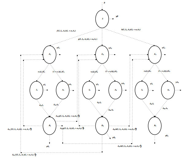
We investigate the behavior of a complex three-strain model with a generalized incidence rate. The incidence rate is an essential aspect of the model as it determines the number of new infections emerging. The mathematical model comprises thirteen nonlinear ordinary differential equations with susceptible, exposed, symptomatic, asymptomatic and recovered compartments. The model is well-posed and verified through existence, positivity and boundedness. Eight equilibria comprise a disease-free equilibria and seven endemic equilibrium points following the existence of three strains. The basic reproduction numbers $ \mathfrak{R}_{01} $, $ \mathfrak{R}_{02} $ and $ \mathfrak{R}_{03} $ represent the dominance of strain 1, strain 2 and strain 3 in the environment for new strain emergence. The model establishes local stability at a disease-free equilibrium point. Numerical simulations endorse the impact of general incidence rates, including bi-linear, saturated, Beddington DeAngelis, non-monotone and Crowley Martin incidence rates.

References

[1]	W. O. Kermack, A. G. McKendrick, A contribution to the mathematical theory of epidemics, Proc. R. Soc. Lond. A., 115 (1927), 700–721. https://doi.org/10.1098/rspa.1927.0118 doi: 10.1098/rspa.1927.0118
[2]	J. Murray, Mathematical Biology, Springer-Verlag, Heidelberg, 1 (2002).
[3]	F. Brauer, C. C. Chavez, Z. Feng, Mathematical Models in Epidemiology, Springer, 32 (2019). https://doi.org/10.1007/978-1-4939-9828-9
[4]	S. Garmer, R. Lynn, D. Rossi, A. Capaldi, Multistrain infections in metapopulations, Spora, 1 (2015), 17–27. https://doi.org/10.30707/SPORA1.1Garmer doi: 10.30707/SPORA1.1Garmer
[5]	E. Cirulli, D. Goldstein, Uncovering the roles of rare variants in common disease through whole-genome sequencing, Nat. Rev. Genet., 11 (2010), 415–425. https://doi.org/10.1038/nrg2779 doi: 10.1038/nrg2779
[6]	M. Cascella, M. Rajnik, A. Aleem, Features, Evaluation, and Treatment of Coronavirus (COVID-19), StatPearls Publishing, 2022.
[7]	Z. Yaagoub, K. Allali, Global stability of multi-strain SEIR epidemic model with vaccination strategy, Math. Comput. Appl., 28 (2023), 9. https://doi.org/10.3390/mca28010009 doi: 10.3390/mca28010009
[8]	T. Sardar, I. Ghosh, X. Rodó, J. Chattopadhyay, A realistic two-strain model for MERS-CoV infection uncovers the high risk for epidemic propagation, PLoS Neglected Trop. Dis., 14 (2020), e0008065. https://doi.org/10.1371/journal.pntd.0008065 doi: 10.1371/journal.pntd.0008065
[9]	M. A. Kuddus, E. S. McBryde, A. I. Adekunle, M. T. Meehan, Analysis and simulation of a two-strain disease model with nonlinear incidence, Chaos Solitons Fractals, 155 (2022). https://doi.org/10.1016/j.chaos.2021.111637 doi: 10.1016/j.chaos.2021.111637
[10]	V. P. Bajiya, J. P. Tripathi, V. Kakkar, J. Wang, G. Sun, Global dynamics of a multi-group SEIR epidemic model with infection age, Chin. Ann. Math. Ser. B, 42 (2021), 833–860. https://doi.org/10.1007/s11401-021-0294-1 doi: 10.1007/s11401-021-0294-1
[11]	E. F. Arruda, S. S. Das, C. M. Dias, D. H. Pastore, Modelling and optimal control of multi strain epidemics, with application to COVID-19, PLoS ONE, 16 (2021). https://doi.org/10.1371/journal.pone.0257512 doi: 10.1371/journal.pone.0257512
[12]	S. Ghosh, M. Banerjee, A multi-strain model for COVID-19, in Applied Analysis, Applied Analysis, Optimization and Soft Computing, 2022. https://doi.org/10.1007/978-981-99-0597-3_10
[13]	S. W. X. Ong, C. J. Chiew, L. W. Ang, T. Mak, L. Cui, M. P. H. S. Toh, et al., Clinical and virological features of severe acute respiratory syndrome coronavirus 2 (SARS-CoV-2) variants of concern: A retrospective cohort study comparing B.1.1.7 (Alpha), B.1.351 (Beta), and B.1.617.2 (Delta), Clin. Infect. Dis., 75 (2021), e1128–e1136. https://doi.org/10.1093/cid/ciab721 doi: 10.1093/cid/ciab721
[14]	M. Massard, R. Eftimie, A. Perasso, B. Saussereau, A multi-strain epidemic model for COVID-19 with infected and asymptomatic cases: application to French data, J. Theor. Biol., 545 (2022), 111117. https://doi.org/10.1016/j.jtbi.2022.111117 doi: 10.1016/j.jtbi.2022.111117
[15]	Z. Abreu, G. Cantin, C. J. Silva, Analysis of a COVID-19 compartmental model: a mathematical and computational approach, Math. Biosci. Eng., 18 (2021), 7979–7998. https://doi.org/10.3934/mbe.2021396 doi: 10.3934/mbe.2021396
[16]	World Health Organization, Coronavirus World Health Organization 19. Available from: https://www.who.int/health-topics/coronavirus.
[17]	Center for Disease Control and prevention (CDC). Available from: https://www.cdc.gov/coronavirus/2019-ncov/variants/variant-classifications.html
[18]	National Center for Biotechnology Information (NCBI). Available from: https://www.ncbi.nlm.nih.gov/activ.
[19]	G. Rohith, K. B. Devika, Dynamics and control of COVID-19 pandemic with nonlinear incidence rates, Nonlinear Dyn., 101 (2020), 2013–2026. https://doi.org/10.1007/s11071-020-05774-5 doi: 10.1007/s11071-020-05774-5
[20]	S. Ruan, W. Wang, Dynamical behavior of an epidemic model with a nonlinear incidence rate, J. Diff. Equation, 188 (2003), 135–163. https://doi.org/10.1016/S0022-0396(02)00089-X doi: 10.1016/S0022-0396(02)00089-X
[21]	H. W. Hethcote, P. van den Driessche, Some epidemiological models with nonlinear incidence, J. Math. Biol., 29 (1991), 271–287. https://doi.org/10.1007/bf00160539 doi: 10.1007/bf00160539
[22]	G. Huang, Y. Takeuchi, W. Ma, D. Wei, Global stability for delay SIR and SEIR epidemic models with nonlinear incidence rate, Bull. Math. Biol., 72 (2010), 1192–1207. https://doi.org/10.1007/s11538-009-9487-6 doi: 10.1007/s11538-009-9487-6
[23]	W. M. Liu, S. A. Levin, Y. Iwasa, Influence of nonlinear incidence rates upon the behavior of SIRS epidemiological models, J. Math. Biol., 23 (1986), 187–204. https://doi.org/10.1007/BF00276956 doi: 10.1007/BF00276956
[24]	J. Arino, C. C. McCluskey, Effect of a sharp change of the incidence function on the dynamics of a simple disease, J. Bio. Dyn., 4 (2010), 490–505. https://doi.org/10.1080/17513751003793017 doi: 10.1080/17513751003793017
[25]	N. Bellomo, R. Bingham, M. A. J. Chaplain, G. Dosi, G. Forni, D. A. Knopoff, et al., A multiscale model of virus pandemic: Heterogeneous interactive entities in a globally connected world, Math. Models Methods Appl. Sci., 30 (2020), 1591–1651. https://doi.org/10.1142/s0218202520500323 doi: 10.1142/s0218202520500323
[26]	J. J. Wang, J. Z. Zhang, Z. Jin, Analysis of an SIR model with bilinear incidence rate, Nonlinear Anal. Real World Appl., 11 (2010), 2390–2402. https://doi.org/10.1016/j.nonrwa.2009.07.012 doi: 10.1016/j.nonrwa.2009.07.012
[27]	O. Khyar, K. Allali, Global dynamics of a multi-strain SEIR epidemic model with general incidence rates: application to COVID-19 pandemic, Nonlinear Dyn., (2020), 1–21. https://doi.org/10.1007/s11071-020-05929-4 doi: 10.1007/s11071-020-05929-4
[28]	X. Liu, L. Yang, Stability analysis of an SEIQV epidemic model with saturated incidence rate, Nonlinear Anal. Real World Appl., 13 (2012), 2671–2679. https://doi.org/10.1016/j.nonrwa.2012.03.010 doi: 10.1016/j.nonrwa.2012.03.010
[29]	A. Kaddar, On the dynamics of a delayed SIR epidemic model with a modified saturated incidence rate, Electron. J. Differ. Equation, 13 (2009), 1–7.
[30]	Y. Zhao, D. Jiang, The threshold of a stochastic SIRS epidemic model with saturated incidence, Appl. Math. Lett., 34 (2014), 90–93. https://doi.org/10.3934/dcdsb.2015.20.1277 doi: 10.3934/dcdsb.2015.20.1277
[31]	X. Q. Liu, S. M. Zhong, B. D. Tian, F. X. Zheng, Asymptotic properties of a stochastic predator-prey model with Crowley–Martin functional response, J. Appl. Math. Comput., 43 (2013), 479–490. https://doi.org/10.1007/s12190-013-0674-0 doi: 10.1007/s12190-013-0674-0
[32]	J. R. Beddington, Mutual interference between parasites or predators and its effect on searching efficiency, J. Anim. Ecol., 44 (1975), 331–341. https://doi.org/10.2307/3866 doi: 10.2307/3866
[33]	R. S. Cantrell, C. Cosner, On the dynamics of predator-prey models with the Beddington–DeAngelis functional response, J. Math. Anal. Appl., 257 (2001), 206–222. https://doi.org/10.1006/JMAA.2000.7343 doi: 10.1006/JMAA.2000.7343
[34]	X. Zhou, J. Cui, Global stability of the viral dynamics with Crowley–Martin functional response, Bull. Korean Math. Soc., 48 (2011), 555–574. https://doi.org/10.1002/mma.3078 doi: 10.1002/mma.3078
[35]	K. Hattaf, N. Yousfi, A. Tridane, Mathematical analysis of a virus dynamics model with general incidence rate and cure rate, Nonlinear Anal. Real World Appl., 13 (2012), 1866–1872. https://doi.org/10.1016/j.nonrwa.2011.12.015 doi: 10.1016/j.nonrwa.2011.12.015
[36]	K. Hattaf, M. Mahrouf, J. Adnani, N. Yousfi, Qualitative analysis of a stochastic epidemic model with specific functional response and temporary immunity, Phys. A., 490 (2018), 591–600. https://doi.org/10.1016/j.physa.2017.08.043 doi: 10.1016/j.physa.2017.08.043
[37]	K. Hattaf, N. Yousfi, Global dynamics of a delay reaction–diffusion model for viral infection with specific functional response, Comput. Appl. Math., 34 (2015), 807–818. https://doi.org/10.1007/s40314-014-0143-x doi: 10.1007/s40314-014-0143-x
[38]	K. Hattaf, N. Yousfi, A. Tridane, Stability analysis of a virus dynamics model with general incidence rate and two delays, Appl. Math. Comput., 221 (2013), 514–521. https://doi.org/10.1016/j.amc.2013.07.005 doi: 10.1016/j.amc.2013.07.005
[39]	M. K. Singh, Anjali, Mathematical modeling and analysis of seqiahr model: Impact of quarantine and isolation on COVID-19, App. App. Math., 17 (2022), 146–171.
[40]	S. Sharma, V. Volpert, M. Banerjee, Extended SEIQR type model for covid-19 epidemic and data analysis, Math. Biosci. Eng., (2020), 7562–7604. https://doi.org/10.3934/mbe.2020386 doi: 10.3934/mbe.2020386
[41]	P. Kim, S. M. Gordon, M. M. Sheehan, M. B. Rothberg, Duration of severe acute respiratory syndrome Coronavirus 2 natural immunity and protection against the Delta variant: A retrospective cohort study, Clin. Infect. Dis., 75 (2022), 185–190. https://doi.org/10.1093/cid/ciab999 doi: 10.1093/cid/ciab999
[42]	P. Van den Driessche, J. Watmough, Reproduction numbers and sub-threshold endemic equilibria for compartmental models of disease transmission, Math. Biosci., 180 (2002), 29–48. https://doi.org/10.1016/s0025-5564(02)00108-6 doi: 10.1016/s0025-5564(02)00108-6
[43]	D. Bentaleb, S. Amine, Lyapunov function and global stability for a two-strain SEIR model with bilinear and non-monotone, Int. J. Biomath., 12 (2019). https://doi.org/10.1142/S1793524519500219 doi: 10.1142/S1793524519500219
[44]	F. G. Ball, E. S. Knock, P. D. O'Neil, Control of emerging infectious diseases using responsive imperfect vaccination and isolation, Math. Biosci., 216 (2008), 100–113. https://doi.org/10.1016/j.mbs.2008.08.008 doi: 10.1016/j.mbs.2008.08.008
[45]	C. Castilho, Optimal control of an epidemic through educational campaigns, Electron. J. Differ. Equation, (2006), 1–11.

Reader Comments

Your name:*

Email:*
© 2023 the Author(s), licensee AIMS Press. This is an open access article distributed under the terms of the Creative Commons Attribution License (http://creativecommons.org/licenses/by/4.0)