Contrast U-Net driven by sufficient texture extraction for carotid plaque detection

WenJun Zhou; Tianfei Wang; Yuhang He; Shenghua Xie; Anguo Luo; Bo Peng; Lixue Yin; WenJun Zhou; Tianfei Wang; Yuhang He; Shenghua Xie; Anguo Luo; Bo Peng; Lixue Yin

doi:10.3934/mbe.2023697

Mathematical Biosciences and Engineering

2023, Volume 20, Issue 9: 15623-15640. doi: 10.3934/mbe.2023697

Previous Article Next Article

Research article

Contrast U-Net driven by sufficient texture extraction for carotid plaque detection

1.
Ultrasound in Cardiac Electrophysiology and Biomechanics Key Laboratory of Sichuan Province, Sichuan Provincial People's Hospital, University of Electronic Science and Technology of China, Chengdu 611731, China
2.
School of Computer Science, Southwest Petroleum University, Chengdu 610500, China

Received: 20 March 2023 Revised: 02 July 2023 Accepted: 10 July 2023 Published: 28 July 2023

Ischemic heart disease or stroke caused by the rupture or dislodgement of a carotid plaque poses a huge risk to human health. To obtain accurate information on the carotid plaque characteristics of patients and to assist clinicians in the determination and identification of atherosclerotic areas, which is one significant foundation work. Existing work in this field has not deliberately extracted texture information of carotid from the ultrasound images. However, texture information is a very important part of carotid ultrasound images. To make full use of the texture information in carotid ultrasound images, a novel network based on U-Net called Contrast U-Net is designed in this paper. First, the proposed network mainly relies on a contrast block to extract accurate texture information. Moreover, to make the network better learn the texture information of each channel, the squeeze-and-excitation block is introduced to assist in the jump connection from encoding to decoding. Experimental results from intravascular ultrasound image datasets show that the proposed network can achieve superior performance compared with other popular models in carotid plaque detection.
- carotid plaque,
- texture information,
- Semantic Segmentation,
- contrast block,
- Contrast U-Net
Citation: WenJun Zhou, Tianfei Wang, Yuhang He, Shenghua Xie, Anguo Luo, Bo Peng, Lixue Yin. Contrast U-Net driven by sufficient texture extraction for carotid plaque detection[J]. Mathematical Biosciences and Engineering, 2023, 20(9): 15623-15640. doi: 10.3934/mbe.2023697

Related Papers:

Abstract

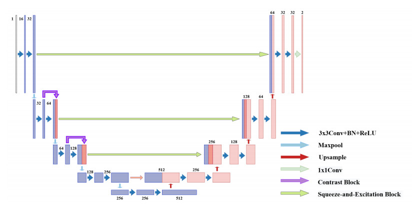
Ischemic heart disease or stroke caused by the rupture or dislodgement of a carotid plaque poses a huge risk to human health. To obtain accurate information on the carotid plaque characteristics of patients and to assist clinicians in the determination and identification of atherosclerotic areas, which is one significant foundation work. Existing work in this field has not deliberately extracted texture information of carotid from the ultrasound images. However, texture information is a very important part of carotid ultrasound images. To make full use of the texture information in carotid ultrasound images, a novel network based on U-Net called Contrast U-Net is designed in this paper. First, the proposed network mainly relies on a contrast block to extract accurate texture information. Moreover, to make the network better learn the texture information of each channel, the squeeze-and-excitation block is introduced to assist in the jump connection from encoding to decoding. Experimental results from intravascular ultrasound image datasets show that the proposed network can achieve superior performance compared with other popular models in carotid plaque detection.

References

[1]	G. K. Hansson, Inflammation, atherosclerosis, and coronary artery disease, N. Engl. J. Med., 352 (2005), 1685–1695. http://doi.org/10.1056/NEJMra043430 doi: 10.1056/NEJMra043430
[2]	R. Virmani, F. D. Kolodgie, A. P. Burke, A. V. Finn, H. K. Gold, T. N. Tulenko, et al., Atherosclerotic plaque progression and vulnerability to rupture: angiogenesis as a source of intraplaque hemorrhage, Arterioscler. Thromb. Vasc. Biol., 25 (2005), 2054–2061. http://doi.org/10.1090/S0894-0347-1992-1124979-1 doi: 10.1090/S0894-0347-1992-1124979-1
[3]	B. Smitha, Joseph K. Paul, Fractal and multifractal analysis of atherosclerotic plaque in ultrasound images of the carotid artery, Chaos Solitons Fractals, 123 (2019), 91–100, https://doi.org/10.1016/j.chaos.2019.03.041 doi: 10.1016/j.chaos.2019.03.041
[4]	M. Biswas, L. Saba, T. Omerzu, A. M. Johri, N. N. Khanna, K. Viskovic, et al., A review on joint carotid intima-media thickness and plaque area measurement in ultrasound for cardiovascular/stroke risk monitoring: Artificial intelligence framework, J Digit Imaging, 34 (2021), 581–604. http://doi.org/10.1007/s10278-021-00461-2 doi: 10.1007/s10278-021-00461-2
[5]	Y. Li, S. Zheng, J. Zhang, F. Wang, X. Liu, W. He, Advance ultrasound techniques for the assessment of plaque vulnerability in symptomatic and asymptomatic carotid stenosis: A multimodal ultrasound study, Cardiovasc. Diagn. Ther., 11 (2021), 28. http://doi.org/10.21037/cdt-20-876 doi: 10.21037/cdt-20-876
[6]	O. Ronneberger, P. Fischer, T. Brox, U-net: Convolutional networks for biomedical image segmentation, in Medical Image Computing and Computer-Assisted Intervention – MICCAI 2015, 9351 (2015). http://doi.org/10.1007/978-3-319-24574-4_28
[7]	Ö. Çiçek, A. Abdulkadir, S. S. Lienkamp, T. Brox, O. Ronneberger, 3d u-net: Learning dense volumetric segmentation from sparse annotation, in Medical Image Computing and Computer-Assisted Intervention–MICCAI 2016: 19th International Conference, (2016), 424–432. https://doi.org/10.48550/arXiv.1606.06650
[8]	F. Milletari, N. Navab, S. A. Ahmadi, V-net: Fully convolutional neural networks for volumetric medical image segmentation, in 2016 fourth international conference on 3D vision (3DV), (2016), 565–571. https://doi.org/10.1109/3DV.2016.79
[9]	Z. Zhou, M. M. Rahman Siddiquee, N. Tajbakhsh, J. Liang, Unet++: A nested u-net architecture for medical image segmentation, in Deep learning in medical image analysis and multimodal learning for clinical decision support, Springer, (2018), 3–11. http://doi.org/10.1007/978-3-030-00889-5_1
[10]	F. Isensee, J. Petersen, A. Klein, D. Zimmerer, P. F. Jaeger, S. Kohl, et al., nnu-net: Self-adapting framework for u-net-based medical image segmentation, preprint, arXiv: 1809.10486.
[11]	O. Oktay, J. Schlemper, L. L. Folgoc, M. J. Lee, M. P. Heinrich, K. Misawa, et al., Attention u-net: Learning where to look for the pancreas, preprint, arXiv: 1804.03999.
[12]	H. Chen, X. Qi, L. Yu, P. A. Heng, Dcan: deep contour-aware networks for accurate gland segmentation, in Proceedings of the IEEE conference on Computer Vision and Pattern Recognition, (2016), 2487–2496. https://doi.org/10.1016/j.media.2016.11.004
[13]	E. Shelhamer, J. Long, T. Darrell, Fully convolutional networks for semantic segmentation, IEEE Trans. Pattern Anal. Mach. Intell., 39 (2017), 640–651. http://doi.org/10.1109/TPAMI.2016.2572683 doi: 10.1109/TPAMI.2016.2572683
[14]	Z. Gu, J. Cheng, H. Fu, K. Zhou, H. Hao, Y. Zhao, et al., Ce-net: Context encoder network for 2d medical image segmentation, IEEE Trans. Med. Imaging., 38 (2019), 2281–2292. http://doi.org/10.1109/TMI.2019.2903562 doi: 10.1109/TMI.2019.2903562
[15]	M. Z. Alom, M. Hasan, C. Yakopcic, T. M. Taha, V. K. Asari, Recurrent residual convolutional neural network based on u-net (r2u-net) for medical image segmentation, preprint, arXiv: 1802.06955.
[16]	Z. Wang, N. Zou, D. Shen, S. Ji, Non-local u-nets for biomedical image segmentation, in Proceedings of the AAAI Conference on Artificial Intelligence, (2020), 6315–6322. http://doi.org/10.48550/arXiv.1812.04103
[17]	Y. Dong, Y. Pan, X. Zhao, R. Li, C. Yuan, W. Xu, Identifying carotid plaque composition in mri with convolutional neural networks, in 2017 IEEE International Conference on Smart Computing (SMARTCOMP), (2017), 1–8. http://doi.org/10.1109/SMARTCOMP.2017.7947015
[18]	N. H. Meshram, C. C. Mitchell, S. Wilbrand, R. J. Dempsey, T. Varghese, Deep learning for carotid plaque segmentation using a dilated u-net architecture, Ultrasonic Imaging, 42 (2020), 221–230. http://dx.doi.org/10.1177/0161734620951216 doi: 10.1177/0161734620951216
[19]	M. Xie, Y. Li, Y. Xue, L. Huntress, W. Beckerman, S. A. Rahimi, et al., Two-stage and dual-decoder convolutional u-net ensembles for reliable vessel and plaque segmentation in carotid ultrasound images, in 2020 19th IEEE International Conference on Machine Learning and Applications (ICMLA), (2020), 1376–1381. http://doi.org/10.1109/ICMLA51294.2020.00214
[20]	C. Zhao, A. Vij, S. Malhotra, J. Tang, H. Tang, D. Pienta, et al., Automatic extraction and stenosis evaluation of coronary arteries in invasive coronary angiograms, Comput. Biol. Med., 136 (2021), 104667. https://doi.org/10.1016/j.compbiomed.2021.104667 doi: 10.1016/j.compbiomed.2021.104667
[21]	J. He, Q. Zhu, K. Zhang, P. Yu, J. Tang, An evolvable adversarial network with gradient penalty for covid-19 infection segmentation, Appl. Soft Comput., 113 (2021), 107947. http://doi.org/10.1016/j.asoc.2021.107947 doi: 10.1016/j.asoc.2021.107947
[22]	J. Hu, L. Shen, G. Sun, squeeze-and-excitation networks, in Proceedings of the IEEE Conference on Computer Vision and Pattern Recognition, (2018), 7132–7141. http://dx.doi.org/10.48550/arXiv.1709.01507
[23]	O. Ronneberger, P. Fischer, T. Brox, U-net: Convolutional networks for biomedical image segmentation, in International Conference on Medical image computing and computer-assisted intervention, Springer, (2015), 234–241. http://doi.org/10.1007/978-3-319-24574-4_28
[24]	Y. He, S. Xiang, W. Zhou, B. Peng, R. Wang, L. Li, A novel contrast operator for robust object searching, in 2021 17th International Conference on Computational Intelligence and Security (CIS), (2021), 309–313. http://doi.org/10.1109/CIS54983.2021.00071
[25]	T. Y. Lin, P. Goyal, R. Girshick, K. He, P. Dollár, Focal loss for dense object detection, in Proceedings of the IEEE international conference on computer vision, (2017), 2980–2988. http://doi.org/10.48550/arXiv.1708.02002
[26]	M. Berman, A. R. Triki, M. B. Blaschko, The lovász-softmax loss: A tractable surrogate for the optimization of the intersection-over-union measure in neural networks, in Proceedings of the IEEE conference on computer vision and pattern recognition, (2018), 4413–4421. http://doi.org/10.48550/arXiv.1705.08790
[27]	J. Tang, S. Guo, Q. Sun, Y. Deng, D. Zhou, Speckle reducing bilateral filter for cattle follicle segmentation, BMC Genomics, 11 (2010), 1–9. http://doi.org/10.1186/1471-2164-11-S2-S9 doi: 10.1186/1471-2164-11-S2-S9
[28]	X. Liu, J. Liu, X. Xu, L. Chun, J. Tang, Y. Deng, A robust detail preserving anisotropic diffusion for speckle reduction in ultrasound images, BMC Genomics, 12 (2011), 1–10. http://doi.org/10.1186/1471-2164-12-S5-S14 doi: 10.1186/1471-2164-12-S5-S14
[29]	D. Jha, P. H. Smedsrud, M. A. Riegler, D. Johansen, T. De Lange, P. Halvorsen, et al., Resunet++: An advanced architecture for medical image segmentation, in 2019 IEEE International Symposium on Multimedia (ISM), (2019), 225–2255. http://doi.org/10.1109/ISM46123.2019.00049

Reader Comments

Your name:*

Email:*
© 2023 the Author(s), licensee AIMS Press. This is an open access article distributed under the terms of the Creative Commons Attribution License (http://creativecommons.org/licenses/by/4.0)