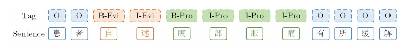
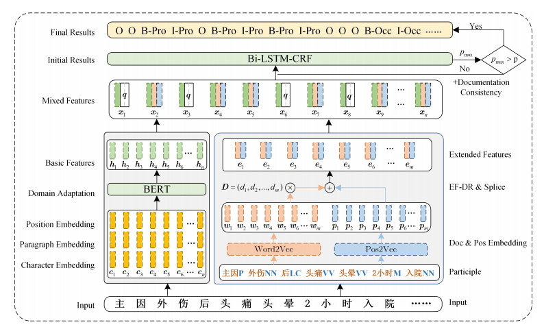
Structured information especially medical events extracted from electronic medical records has extremely practical application value and play a basic role in various intelligent diagnosis and treatment systems. Fine-grained Chinese medical event detection is crucial in the process of structuring Chinese Electronic Medical Record (EMR). The current methods for detecting fine-grained Chinese medical events primarily rely on statistical machine learning and deep learning. However, they have two shortcomings: 1) they neglect to take into account the distribution characteristics of these fine-grained medical events. 2) they overlook the consistency in the distribution of medical events within each individual document. Therefore, this paper presents a fine-grained Chinese medical event detection method, which is based on event frequency distribution ratio and document consistency. To start with, a significant number of Chinese EMR texts are used to adapt the Chinese pre-training model BERT to the domain. Second, based on the fundamental features, the Event Frequency - Event Distribution Ratio (EF-DR) is devised to select distinct event information as supplementary features, taking into account the distribution of events within the EMR. Finally, using EMR document consistency within the model improves the outcome of event detection. Our experiments demonstrate that the proposed method significantly outperforms the baseline model.
Citation: Ruirui Han, Zhichang Zhang, Hao Wei, Deyue Yin. Chinese medical event detection based on event frequency distribution ratio and document consistency[J]. Mathematical Biosciences and Engineering, 2023, 20(6): 11063-11080. doi: 10.3934/mbe.2023489
Structured information especially medical events extracted from electronic medical records has extremely practical application value and play a basic role in various intelligent diagnosis and treatment systems. Fine-grained Chinese medical event detection is crucial in the process of structuring Chinese Electronic Medical Record (EMR). The current methods for detecting fine-grained Chinese medical events primarily rely on statistical machine learning and deep learning. However, they have two shortcomings: 1) they neglect to take into account the distribution characteristics of these fine-grained medical events. 2) they overlook the consistency in the distribution of medical events within each individual document. Therefore, this paper presents a fine-grained Chinese medical event detection method, which is based on event frequency distribution ratio and document consistency. To start with, a significant number of Chinese EMR texts are used to adapt the Chinese pre-training model BERT to the domain. Second, based on the fundamental features, the Event Frequency - Event Distribution Ratio (EF-DR) is devised to select distinct event information as supplementary features, taking into account the distribution of events within the EMR. Finally, using EMR document consistency within the model improves the outcome of event detection. Our experiments demonstrate that the proposed method significantly outperforms the baseline model.

| [1] | J. H. Wang, Research on Information Extraction Method of Chinese Electronic Medical Records, Hunan University, 2016. |
| [2] |
Y. Ahuja, N. Kim, L. Liang, T. Cai, K. Dahal, T. Seyok, et al., Leveraging electronic health records data to predict multiple sclerosis disease activity, Ann. Clin. Transl. Neurol., 8 (2021), 800–810. https://doi.org/10.1002/acn3.51324 doi: 10.1002/acn3.51324

|
| [3] |
A. Geva, S. H. Abman, S. F. Manzi, D. D. Ivy, M. P. Mullen, J. Griffin, et al., Leveraging electronic health records data to predict multiple sclerosis disease activity, J. Am. Med. Inf. Assoc., 27 (2020), 294–300. https://doi.org/10.1093/jamia/ocz194 doi: 10.1093/jamia/ocz194
|
| [4] |
Y. H. Su, C. P. Chao, L. C. Hung, S. F. Sung, P. J. Lee, A natural language processing approach to automated highlighting of new information in clinical notes, Appl. Sci., 10 (2020), 2824. https://doi.org/10.3390/app10082824 doi: 10.3390/app10082824
|
| [5] |
A. Geva, S. H. Abman, S. F. Manzi, D. D. Ivy, M. P. Mullen, J. Griffin, et al., Adverse drug event rates in pediatric pulmonary hypertension: a comparison of real-world data sources, J. Am. Med. Inf. Assoc., 27 (2020), 294–300. https://doi.org/10.1093/jamia/ocz194 doi: 10.1093/jamia/ocz194
|
| [6] |
S. Kulshrestha, D. Dligach, C. Joyce, M. S. Baker, R. Gonzalez, A. P. O'Rourke, et al., Prediction of severe chest injury using natural language processing from the electronic health record, Injury, 52 (2021), 205–212. https://doi.org/10.1016/j.injury.2020.10.094 doi: 10.1016/j.injury.2020.10.094
|
| [7] |
Z. C. Zhang, M. Y. Zhang, T. Zhou, Y. L. Qiu, Pre-trained language model augmented adversarial training network for Chinese clinical event detection, Math. Biosci. Eng., 17 (2020), 2825–2841. https://doi.org/10.3934/mbe.2020157 doi: 10.3934/mbe.2020157
|
| [8] | S. Bethard, L. Derczynski, G. Savova, J. Pustejovsky, M. Verhagen, Semeval-2015 task 6: Clinical tempeval, in Proceedings of the 9th International Workshop on Semantic Evaluation, (2015), 806–814. |
| [9] | S. Bethard, G. Savova, W. T. Chen, L. Derczynski, J. Pustejovsky, M. Verhagen, Semeval-2016 task 12: Clinical tempeval, in Proceedings of the 10th International Workshop on Semantic Evaluation, (2016), 1052–1062. |
| [10] | S. Bethard, G. Savova, M. Palmer, J. Pustejovsky, Semeval-2017 task 12: Clinical tempeval, Proceedings of the 11th International Workshop on Semantic Evaluation, (2017), 565–572. |
| [11] | NegEx, Available from: http://code.google.com/p/negex/. |
| [12] | P. Szolovits, Adding a medical lexicon to an English parser, in AMIA Annual Symposium Proceedings, (2003), 639. |
| [13] | T. C. Sibanda, Was the Patient Cured?: Understanding Semantic Categories and their Relationship in Patient Records, Massachusetts Institute of Technology, 2006. |
| [14] | Y. Sun, A. Nguyen, L. Sitbon, S. Geva, Rule-based approach for identifying assertions in clinical free-text data, in Proceedings of 15th Australasian Document Computing Symposium, (2010), 93–96. |
| [15] |
A. L. Minard, A. L. Ligozat, A. B. Abacha, D. Bernhard, B. Cartoni, L. Deléger, et al., Hybrid methods for improving information access in clinical documents: concept, assertion, and relation identification, J. Am. Med. Inf. Assoc., 18 (2011), 588–593. https://doi.org/10.1136/amiajnl-2011-000154 doi: 10.1136/amiajnl-2011-000154
|
| [16] | J. Lafferty, A. McCallum, F. Pereira, Conditional random fields: Probabilistic models for segmenting and labeling sequence data, in Proceedings of the 18th International Conference on Machine Learning 2001 (ICML 2001), 8 (2001), 282–289. https://doi.org/10.1109/ICIP.2012.6466940 |
| [17] |
C. Cortes, V. Vladimir, Support-vector networks, Mach. Learn., 20 (1995), 273–297. https://doi.org/10.1023/A:1022627411411 doi: 10.1023/A:1022627411411
|
| [18] |
Y. Xu, Y. N. Wang, T. R. Liu, J. Tsujii, E. I. Chang, An end-to-end system to identify temporal relation in discharge summaries: 2012 i2b2 challenge, J. Am. Med. Inf. Assoc., 20 (2013), 849–858. https://doi.org/10.1136/amiajnl-2012-001607 doi: 10.1136/amiajnl-2012-001607
|
| [19] |
K. Roberts, B. Rink, S. M. Harabagiu, A flexible framework for recognizing events, temporal expressions, and temporal relations in clinical text, J. Am. Med. Inf. Assoc., 20 (2013), 867–875. https://doi.org/10.1136/amiajnl-2013-001619 doi: 10.1136/amiajnl-2013-001619
|
| [20] |
Y. K. Lin, H. Chen, R. A. Brown, MedTime: A temporal information extraction system for clinical narratives, J. Biomed. Inf., 46 (2013), 20–28. https://doi.org/10.1016/j.jbi.2013.07.012 doi: 10.1016/j.jbi.2013.07.012
|
| [21] |
J. D'Souza, V. NgY, Classifying temporal relations in clinical data: a hybrid, knowledge-rich approach, J. Biomed. Inf., 46 (2013), 29–39. https://doi.org/10.1016/j.jbi.2013.08.003 doi: 10.1016/j.jbi.2013.08.003
|
| [22] | Z. H. Huang, W. Xu, K. Yu, Bidirectional LSTM-CRF models for sequence tagging, preprint, arXiv: math/1508.01991. https://doi.org/10.48550/arXiv.1508.01991 |
| [23] | Y. Zhang, J. Yang, Chinese NER using lattice LSTM, preprint, arXiv: math/1805.02023. https://doi.org/10.48550/arXiv.1805.02023 |
| [24] | W. Liu, T. G. Xu, Q. H. Xu, J. Y. Song, Y. R. Zu, An encoding strategy based word-character LSTM for Chinese NER, in Proceedings of the 2019 Conference of the North American Chapter of the Association for Computational Linguistics, 1 (2019), 2379–2389. https://doi.org/10.18653/v1/N19-1247 |
| [25] | B. Ji, R. Liu, S. S. Li, J. T. Tang, Q. Li, W. S. Xu, A BILSTM-CRF method to Chinese electronic medical record named entity recognition, in Proceedings of the 2018 International Conference on Algorithms, 48 (2018), 1–6. https://doi.org/10.1145/3302425.3302465 |
| [26] |
B. Ji, R. Liu, S. S. Li, J. T. Tang, Q. Li, W. S. Xu, A joint extraction method for Chinese medical events, Comput. Sci., 48 (2018), 287–293. https://doi.org/10.48550/arXiv.1907.11692 doi: 10.48550/arXiv.1907.11692
|
| [27] | J. Devlin, M. W. Chang, K. Lee, K. Toutanova, Bert: Pre-training of deep bidirectional transformers for language understanding, preprint, arXiv: math/1810.04805. https://doi.org/10.48550/arXiv.1810.04805 |
| [28] | Y. H. Liu, M. Ott, N. Goyal, J. F. Du, M. Joshi, D. Q. Chen, et al., Roberta: A robustly optimized bert pretraining approach, preprint, arXiv: math/1907.11692. https://doi.org/10.48550/arXiv.1907.11692 |
| [29] | X. N. Zhang, CCKS2020 medical event extraction based on named entity recognition. Available from: https://bj.bcebos.com/v1/conference/ccks2020/eval_paper/ccks2020_eval_paper_3_2_2.pdf. |
| [30] | S. T. Dai, Small sample medical event extraction based on pre-trained language model. Available from: https://bj.bcebos.com/v1/conference/ccks2020/eval_paper/ccks2020_eval_paper_3_2_1.pdf. |
| [31] | L. Y. Yang, J. Q. Li, Z. C. Zhu, X. M. Dong, F. Akhtar, Chinese medical event extraction based on hybrid neural network, in 2022 IEEE 46th Annual Computers, (2022), 1420–1425. https://doi.org/10.1109/COMPSAC54236.2022.00225 |
| [32] | L. Hou, P. Li, Q. Zhu, Study of event recognition based on CRFs and cross-event, Comput. Eng., 38 (2012), 191–195. |
| [33] |
J. B. Xia, C. Y. Fang, X. Zhang, A novel feature selection strategy for enhanced biomedical event extraction using the Turku system, BioMed Res. Int., 2014 (2014), 1–12. https://doi.org/10.1155/2014/205239 doi: 10.1155/2014/205239
|
| [34] | C. Wang, P. Zhai, Y. Fang, Chinese medical event detection based on feature extension and document consistency, in 2020 5th International Conference on Automation, Control and Robotics Engineering, (2020), 753–758. https://doi.org/10.1109/CACRE50138.2020.9230246 |
| [35] | I. Turc, M. W. Chang, K. Lee, K. Toutanova, Well-read students learn better: On the importance of pre-training compact models, preprint, arXiv: math/1908.08962. https://doi.org/10.48550/arXiv.1908.08962 |
| [36] | LTP, Available from: http://ltp.ai/. |
| [37] | S. Gururangan, A. Marasović, S. Swayamdipta, K. Lo, I. Beltagy, D. Downey, et al., Don't stop pretraining: Adapt language models to domains and tasks, preprint, arXiv: math/2004.10964. https://doi.org/10.48550/arXiv.2004.10964 |
| [38] | Q. Le, T. Mikolov, Distributed representations of sentences and documents, in International Conference on Machine Learning, 32 (2014), 1188–1196. |
| [39] | M. Y. Zhang, Research on Time Series Information Extraction Technology of Clinical Medical Events Based on Electronic Medical Records, Northwest Normal University, 2021. https://doi.org/10.27410/d.cnki.gxbfu.2021.001837 |
Figures(4) / Tables(6)

Ruirui Han, Zhichang Zhang, Hao Wei, Deyue Yin. Chinese medical event detection based on event frequency distribution ratio and document consistency[J]. Mathematical Biosciences and Engineering, 2023, 20(6): 11063-11080. doi: 10.3934/mbe.2023489


 DownLoad: