Accurate depiction of individual teeth from CBCT images is a critical step in the diagnosis of oral diseases, and the traditional methods are very tedious and laborious, so automatic segmentation of individual teeth in CBCT images is important to assist physicians in diagnosis and treatment. TransUNet has achieved success in medical image segmentation tasks, which combines the advantages of Transformer and CNN. However, the skip connection taken by TransUNet leads to unnecessary restrictive fusion and also ignores the rich context between adjacent keys. To solve these problems, this paper proposes a context-transformed TransUNet++ (CoT-UNet++) architecture, which consists of a hybrid encoder, a dense connection, and a decoder. To be specific, a hybrid encoder is first used to obtain the contextual information between adjacent keys by CoTNet and the global context encoded by Transformer. Then the decoder upsamples the encoded features by cascading upsamplers to recover the original resolution. Finally, the multi-scale fusion between the encoded and decoded features at different levels is performed by dense concatenation to obtain more accurate location information. In addition, we employ a weighted loss function consisting of focal, dice, and cross-entropy to reduce the training error and achieve pixel-level optimization. Experimental results demonstrate that the proposed CoT-UNet++ method outperforms the baseline models and can obtain better performance in tooth segmentation.
Citation: Yijun Yin, Wenzheng Xu, Lei Chen, Hao Wu. CoT-UNet++: A medical image segmentation method based on contextual transformer and dense connection[J]. Mathematical Biosciences and Engineering, 2023, 20(5): 8320-8336. doi: 10.3934/mbe.2023364
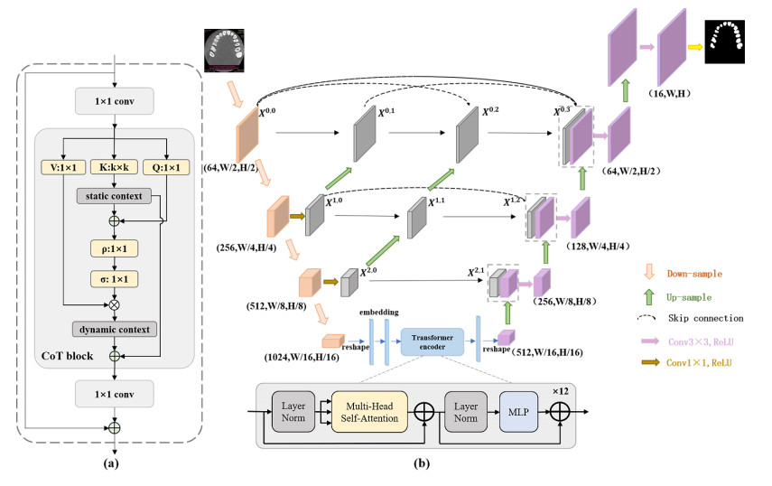
Accurate depiction of individual teeth from CBCT images is a critical step in the diagnosis of oral diseases, and the traditional methods are very tedious and laborious, so automatic segmentation of individual teeth in CBCT images is important to assist physicians in diagnosis and treatment. TransUNet has achieved success in medical image segmentation tasks, which combines the advantages of Transformer and CNN. However, the skip connection taken by TransUNet leads to unnecessary restrictive fusion and also ignores the rich context between adjacent keys. To solve these problems, this paper proposes a context-transformed TransUNet++ (CoT-UNet++) architecture, which consists of a hybrid encoder, a dense connection, and a decoder. To be specific, a hybrid encoder is first used to obtain the contextual information between adjacent keys by CoTNet and the global context encoded by Transformer. Then the decoder upsamples the encoded features by cascading upsamplers to recover the original resolution. Finally, the multi-scale fusion between the encoded and decoded features at different levels is performed by dense concatenation to obtain more accurate location information. In addition, we employ a weighted loss function consisting of focal, dice, and cross-entropy to reduce the training error and achieve pixel-level optimization. Experimental results demonstrate that the proposed CoT-UNet++ method outperforms the baseline models and can obtain better performance in tooth segmentation.

| [1] | W. R. Proffit, H. W. Fields, D. M. Sarver, Contemporary orthodontics: Elsevier Health Sciences, Philadelphia, USA, 2006. |
| [2] |
P. Holm-Pedersen, M. Vigild, I. Nitschke, D. B. Berkey, Dental care for aging populations in Denmark, Sweden, Norway, United kingdom, and Germany, J. Dent. Educ., 69 (2005), 987–997. http://dx.doi.org/10.1002/j.0022-0337.2005.69.9.tb03995.x doi: 10.1002/j.0022-0337.2005.69.9.tb03995.x

|
| [3] |
C. Tian, Y. Zhang, W. Zuo, C. Lin, D. Zhang, Y. Yuan, A heterogeneous group CNN for image super-resolution, IEEE Trans. Neural Netw. Learn. Syst., 2022. https://doi.org/10.1109/TNNLS.2022.3210433 doi: 10.1109/TNNLS.2022.3210433
|
| [4] |
C. Tian, Y. Yuan, S. Zhang, C. Lin, W. Zuo, D. Zhang, Image super-resolution with an enhanced group convolutional neural network, Neural Netw., 153 (2022). https://doi.org/10.1109/TCSVT.2022.3175959 doi: 10.1109/TCSVT.2022.3175959
|
| [5] |
C. Tian, Y. Xu, Z. Li, W. Zuo, L. Fei, H. Liu, Attention-guided CNN for image denoising, Neural Netw., 124 (2020), 117–129. https://doi.org/10.1016/j.neunet.2019.12.024 doi: 10.1016/j.neunet.2019.12.024
|
| [6] |
T. Huang, X. Ben, C. Gong, B. Zhang, R. Yan, Q. Wu, Enhanced spatial-temporal salience for cross-view gait recognition, IEEE Trans. Circuits Syst. Video Technol., 32 (2022), 6967–6980. https://doi.org/10.1109/TCSVT.2022.3175959 doi: 10.1109/TCSVT.2022.3175959
|
| [7] |
X. Ben, C. Gong, P. Zhang, X. Jia, Q. Wu, W. Meng, Coupled patch alignment for matching cross-view gaits, IEEE Trans. Image Process., 28 (2019), 3142–3157. https://doi.org/10.1109/tip.2019.2894362 doi: 10.1109/tip.2019.2894362
|
| [8] |
Y. Guo, B. Li, X. Ben, Y. Ren, J. Zhang, R. Yan, et al., A magnitude and angle combined optical flow feature for microexpression spotting, IEEE Multimedia, 28 (2021), 29–39. https://doi.org/10.1109/MMUL.2021.3058017 doi: 10.1109/MMUL.2021.3058017
|
| [9] |
B. Zhang, R. Wang, X. Wang, J. Han, R. Ji, Modulated convolutional Networks, IEEE Trans/ Neural Netw. Learn. Syst., 2021. https://doi.org/10.1109/TNNLS.2021.3060830 doi: 10.1109/TNNLS.2021.3060830
|
| [10] |
T. Zhou, J. Si, L. Wang, C. Xu, Automatic detection of underwater small targets using forward-looking sonar images, IEEE Trans. Geosci. Remote Sens., 60 (2022), 1–12. https://doi.org/10.1109/TGRS.2022.3181417 doi: 10.1109/TGRS.2022.3181417
|
| [11] | C. Yu, C. Gao, J. Wang, et al., BiSeNet V2: Bilateral Network with Guided Aggregation for Real-Time Semantic Segmentation. in International Journal of Computer Vision, 129 (2021), 3051–3068. https://doi.org/10.1007/s11263-021-01515-2 |
| [12] | X. Zhong, S. Tu, X. Ma, et al., Rainy WCity: A Real Rainfall Dataset with Diverse Conditions for Semantic Driving Scene Understanding. in International Joint Conference on Artificial Intelligence, (2022), 1743-1749. https://doi.org/10.24963/ijcai.2022/243 |
| [13] | O. Ronneberger, P. Fischer, T. Brox, U-net: Convolutional networks for biomedical image segmentation, in International Conference on Medical Image Computing and Computer-Assisted Intervention, (2015), 234–241. https://doi.org/10.1007/978-3-319-24574-4 |
| [14] | F. Milletari, N. Navab, S. A. Ahmadi, V-net: Fully convolutional neural networks for volumetric medical image segmentation, in 2016 Fourth International Conference on 3D Vision (3DV). (2016), 565–571. https://doi.org/10.1109/3DV.2016.79 |
| [15] | Ö. Çiçek, A. Abdulkadir, S. S. Lienkamp, T. Brox, O. Ronneberger, 3D U-Net: learning dense volumetric segmentation from sparse annotation, in International Conference on Medical Image Computing and Computer-Assisted Intervention, (2016), 424–432. https://doi.org/10.1007/978-3-319-46723-8_49 |
| [16] | L. Yu, J. Z. Cheng, Q. Dou, X. Yang, H. Chen, J. Qin, et al., Automatic 3D cardiovascular MR segmentation with densely-connected volumetric convnets, in International Conference on Medical Image Computing and Computer-Assisted Intervention, (2017), 287–295. https://doi.org/10.48550/arXiv.1708.00573 |
| [17] |
X. Li, H. Chen, X. Qi, Q. Dou, C. W. Fu, P. Heng, H-DenseUNet: hybrid densely connected UNet for liver and tumor segmentation from CT volumes, IEEE Trans. Med. Imaging, 37 (2018), 2663–2674. https://doi.org/10.1109/tmi.2018.2845918 doi: 10.1109/tmi.2018.2845918
|
| [18] | Q. Yu, L. Xie, Y. Wang, Y. Zhou, E. K. Fishman, A. L. Yuille, Recurrent saliency transformation network: Incorporating multi-stage visual cues for small organ segmentation, in Proceedings of the IEEE Conference on Computer Vision and Pattern Recognition, (2018), 8280–8289. https://doi.org/10.1109/CVPR.2018.00864 |
| [19] | Y. Zhou, L. Xie, W. Shen, Y. Wang, E. K. Fishman, A. L. Yuille, A fixed-point model for pancreas segmentation in abdominal CT scans, in International Conference on Medical Image Computing and Computer-assisted Intervention, (2017), 693–701. http://dx.doi.org/10.1007/978-3-319-66182-7_79 |
| [20] | Z. Zhou, M. M. Rahman Siddiquee, N. Tajbakhsh, J. Liang, Unet++: A nested u-net architecture for medical image segmentation, in Deep Learning in Medical Image Analysis and Multimodal Learning for Clinical Decision Support, (2018), 3–11. https://doi.org/10.1007/978-3-030-00889-5_1 |
| [21] | H. Huang, L. Lin, R. Tong, H. Hu, Q. Zhang, Y. Iwamoto, et al., Unet 3+: A full-scale connected unet for medical image segmentation, in ICASSP 2020-2020 IEEE International Conference on Acoustics, Speech and Signal Processing (ICASSP), (2020), 1055–1059. https://doi.org/10.1109/ICASSP40776.2020.9053405 |
| [22] | J. M. J. Valanarasu, V. A. Sindagi, I. Hacihaliloglu, V. M. Patel, Kiu-net: Towards accurate segmentation of biomedical images using over-complete representations, in International Conference on Medical Image Computing and Computer-Assisted Intervention, (2020), 363–373. https://doi.org/10.1007/978-3-030-59719-1_36 |
| [23] |
J. Schlemper, O. Oktay, M. Schaap, M. Heinrich, B. Kainz, B. Glocker, et al., Attention gated networks: Learning to leverage salient regions in medical images, Med. Image Anal., 53 (2019), 197–207. https://doi.org/10.1016/j.media.2019.01.012 doi: 10.1016/j.media.2019.01.012
|
| [24] | X. Wang, R. Girshick, A. Gupta, K. He, Non-local neural networks, in Proceedings of the IEEE Conference on Computer Vision and Pattern Recognition, (2018), 7794–7803. https://doi.org/10.1109/CVPR.2018.00813 |
| [25] |
H. Akhoondali, R. A. Zoroofi, G. Shirani, Rapid automatic segmentation and visualization of teeth in ct-scan data, J. Appl. Sci., 9 (2019), 2031–2044. https://dx.doi.org/10.3923/jas.2009.2031.2044 doi: 10.3923/jas.2009.2031.2044
|
| [26] |
D. X. Ji, S. H. Ong, K. W. C. Foong, A level-set based approach for anterior teeth segmentation in cone beam computed tomography images, Comput. Biol. Med., 50 (2014), 116–128. https://doi.org/10.1016/j.compbiomed.2014.04.006 doi: 10.1016/j.compbiomed.2014.04.006
|
| [27] |
Y. Gan, Z. Xia, J. Xiong, Q. Zhao, Y. Hu, J. Zhang, Toward accurate tooth segmentation from computed tomography images using a hybrid level set model, Med. Phys., 42 (2015), 14–27. https://doi.org/10.1118/1.4901521 doi: 10.1118/1.4901521
|
| [28] |
Y. Pei, X. Ai, H. Zha, T. Xu, G. Ma, 3d exemplar-based random walks for tooth segmentation from cone-beam computed tomography images, Med. Phys., 43 (2016), 5040–5050. https://doi.org/10.1118/1.4960364 doi: 10.1118/1.4960364
|
| [29] |
Sandro Barone, Alessandro Paoli, and ARMANDO VIVIANO Razionale. Ct segmentation of dental shapes by anatomy-driven reformation imaging and b-spline modelling, Int. J. Numer. Methods Biomed. Eng., 32 (2016), e02747. https://doi.org/10.1002/cnm.2747 doi: 10.1002/cnm.2747
|
| [30] | Z. Cui, C. Li, W. Wang, ToothNet: Automatic Tooth Instance Segmentation and Identification From Cone Beam CT Images, in 2019 IEEE/CVF Conference on Computer Vision and Pattern Recognition (CVPR), (2019), 6361–6370. https://doi.org/10.1109/CVPR.2019.00653 |
| [31] | J. Chen, Y. Lu, Q. Yu, X. Luo, E. Adeli, Y. Wang, et al., Transunet: Transformers make strong encoders for medical image segmentation, preprint, arXiv: 2102/04306. |
| [32] | I. Bello, B. Zoph, A. Vaswani, J. Shlens, Q. V. Le, Attention augmented convolutional networks, in Proceedings of the IEEE/CVF International Conference on Computer Vision, (2019), 3286–3295. https://doi.org/10.1109/ICCV.2019.00338 |
| [33] | N. Carion, F. Massa, G. Synnaeve, N. Usunier, A. Kirillov, S. Zagoruyko, End-to-end object detection with transformers, in European Conference on Computer Vision, (2020), 213–229. https://doi.org/10.1007/978-3-030-58452-8_13 |
| [34] | A. Dosovitskiy, L. Beyer, A. Kolesnikov, D. Weissenborn, X. Zhai, T. Unterthiner, An image is worth 16x16 words: Transformers for image recognition at scale, preprint, arXiv: 2010/11929. |
| [35] | Y. Li, Y. Pan, T. Yao, J. Chen, T. Mei, Scheduled sampling in vision-language pretraining with decoupled encoder-decoder network, in Proceedings of the AAAI Conference on Artificial Intelligence, 35 (2021), 8518–8526. http://dx.doi.org/10.1609/aaai.v35i10.17034 |
| [36] | Y. Pan, T. Yao, Y. Li, T. Mei, X-linear attention networks for image captioning, in Proceedings of the IEEE/CVF Conference on Computer Vision and Pattern Recognition, (2020), 10971–10980. https://doi.org/10.1109/CVPR42600.2020.01098 |
| [37] |
P. Ramachandran, N. Parmar, A. Vaswani, I. Bello, A. Levskaya, J. Shlens, Stand-alone self-attention in vision models, Adv. Neural Inform. Process. Syst., 32 (2019), https://doi.org/10.48550/arXiv.1906.05909 doi: 10.48550/arXiv.1906.05909
|
| [38] | H. Zhao, J. Jia, V. Koltun, Exploring self-attention for image recognition, in Proceedings of the IEEE/CVF Conference on Computer Vision and Pattern Recognition, (2020), 10076–10085. https://doi.org/10.1109/CVPR42600.2020.01009 |
| [39] |
Y. Li, T. Yao, Y. Pan, T. Mei, Contextual transformer networks for visual recognition, IEEE Trans. Pattern Anal. Mach. Intell., 2022. https://doi.org/10.48550/arXiv.2107.12292 doi: 10.48550/arXiv.2107.12292
|
| [40] | T. Y. Lin, P. Goyal, R. Girshick, K. He, P. Dollar, Focal loss for dense object detection, in Proceedings of the IEEE International Conference on Computer Vision, (2017), 2980–2988. https://doi.org/10.1109/ICCV.2017.324 |
| [41] | K. He, X. Zhang, S. Ren, J. Sun, Deep residual learning for image recognition, in Proceedings of the IEEE Conference on Computer Vision and Pattern Recognition, (2016), 770–778. https://doi.org/10.1109/CVPR.2016.90 |


Figures(3) / Tables(5)

Yijun Yin, Wenzheng Xu, Lei Chen, Hao Wu. CoT-UNet++: A medical image segmentation method based on contextual transformer and dense connection[J]. Mathematical Biosciences and Engineering, 2023, 20(5): 8320-8336. doi: 10.3934/mbe.2023364


 DownLoad: