Improved bat algorithm for roundness error evaluation problem

Guowen Li; Ying Xu; Chengbin Chang; Sainan Wang; Qian Zhang; Dong An; Guowen Li; Ying Xu; Chengbin Chang; Sainan Wang; Qian Zhang; Dong An

doi:10.3934/mbe.2022437

Mathematical Biosciences and Engineering

2022, Volume 19, Issue 9: 9388-9411. doi: 10.3934/mbe.2022437

Previous Article Next Article

Research article

Improved bat algorithm for roundness error evaluation problem

1.
School of Mechanical Engineering, Shenyang Jianzhu University, Shenyang 110168, China
2.
School of Electro-mechanical Engineering, Guangdong University of Technology, Guangdong 510006, China

Academic Editor: Xiaodong Huang

Received: 11 May 2022 Revised: 10 June 2022 Accepted: 19 June 2022 Published: 27 June 2022

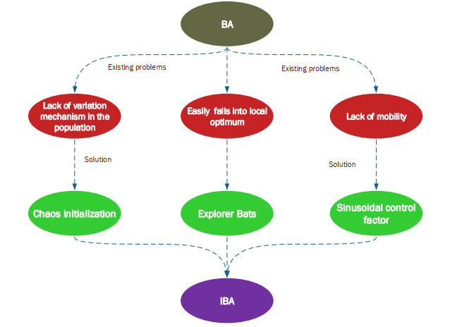
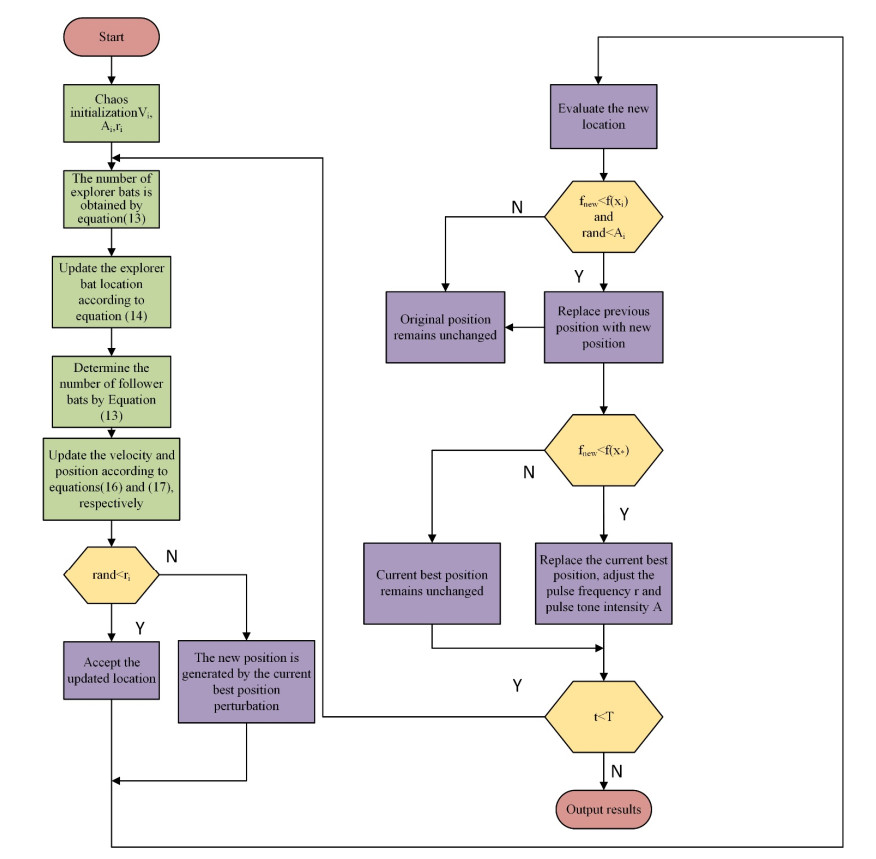
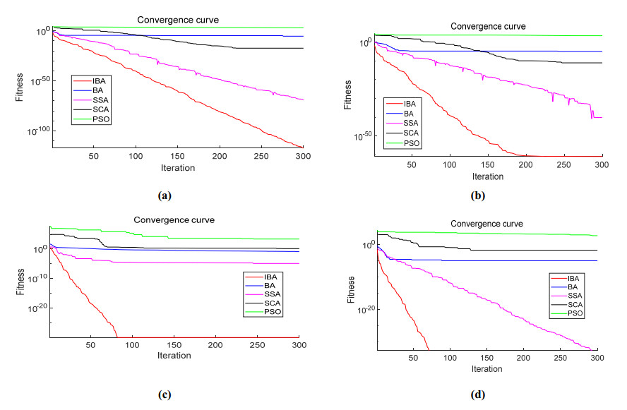
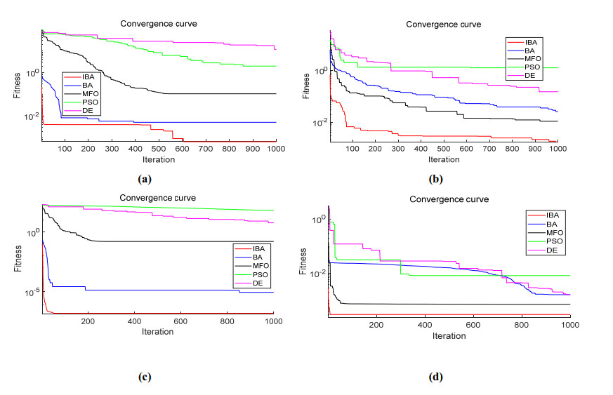
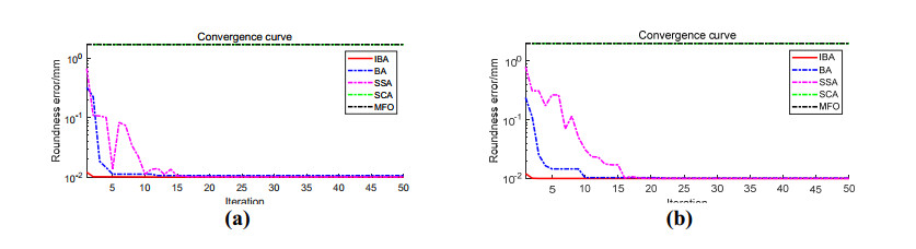
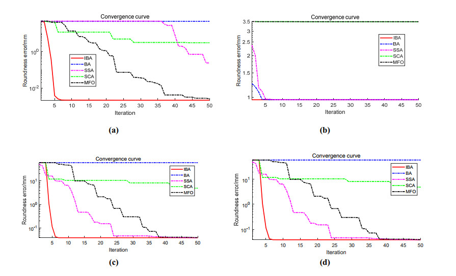
In the production and processing of precision shaft-hole class parts, the wear of cutting tools, machine chatter, and insufficient lubrication can lead to changes in their roundness, which in turn affects the overall performance of the relevant products. To improve the accuracy of roundness error assessments, Bat algorithm (BA) is applied to roundness error assessments. An improved bat algorithm (IBA) is proposed to counteract the original lack of variational mechanisms, which can easily lead BA to fall into local extremes and induce premature convergence. First, logistic chaos initialisation is applied to the initial solution generation to enhance the variation mechanism of the population and improve the solution quality; second, a sinusoidal control factor is added to BA to control the nonlinear inertia weights during the iterative process, and the balance between the global search and local search of the algorithm is dynamically adjusted to improve the optimization-seeking accuracy and stability of the algorithm. Finally, the sparrow search algorithm (SSA) is integrated into BA, exploiting the ability of explorer bats to perform a large range search, so that the algorithm can jump out of local extremes and the convergence speed of the algorithm can be improved. The performance of IBA was tested against the classical metaheuristic algorithm on eight benchmark functions, and the results showed that IBA significantly outperformed the other algorithms in terms of solution accuracy, convergence speed, and stability. Simulation and example verification show that IBA can quickly find the centre of a minimum inclusion region when there are many or few sampling points, and the obtained roundness error value is more accurate than that of other algorithms, which verifies the feasibility and effectiveness of IBA in evaluating roundness errors.
- bat algorithm,
- roundness error,
- convergence speed,
- solution accuracy
Citation: Guowen Li, Ying Xu, Chengbin Chang, Sainan Wang, Qian Zhang, Dong An. Improved bat algorithm for roundness error evaluation problem[J]. Mathematical Biosciences and Engineering, 2022, 19(9): 9388-9411. doi: 10.3934/mbe.2022437

Related Papers:

Abstract

In the production and processing of precision shaft-hole class parts, the wear of cutting tools, machine chatter, and insufficient lubrication can lead to changes in their roundness, which in turn affects the overall performance of the relevant products. To improve the accuracy of roundness error assessments, Bat algorithm (BA) is applied to roundness error assessments. An improved bat algorithm (IBA) is proposed to counteract the original lack of variational mechanisms, which can easily lead BA to fall into local extremes and induce premature convergence. First, logistic chaos initialisation is applied to the initial solution generation to enhance the variation mechanism of the population and improve the solution quality; second, a sinusoidal control factor is added to BA to control the nonlinear inertia weights during the iterative process, and the balance between the global search and local search of the algorithm is dynamically adjusted to improve the optimization-seeking accuracy and stability of the algorithm. Finally, the sparrow search algorithm (SSA) is integrated into BA, exploiting the ability of explorer bats to perform a large range search, so that the algorithm can jump out of local extremes and the convergence speed of the algorithm can be improved. The performance of IBA was tested against the classical metaheuristic algorithm on eight benchmark functions, and the results showed that IBA significantly outperformed the other algorithms in terms of solution accuracy, convergence speed, and stability. Simulation and example verification show that IBA can quickly find the centre of a minimum inclusion region when there are many or few sampling points, and the obtained roundness error value is more accurate than that of other algorithms, which verifies the feasibility and effectiveness of IBA in evaluating roundness errors.

References

[1]	K. Zhang, Minimum zone evolution of circularity error based on an improved Genetic Algorithm, in IEEE 2008 International Conference on Advanced Computer Theory and Engineering (ICACTE), Thailand, (2008), 523–527. https://doi.org/10.1109/ICACTE.2008.168
[2]	J. Luo, Y. Q. Lin, X. M. Liu, P. Zhang, D. Zhou, J. R, Chen, Research on roundness error evaluation based on the improved artificial bee colony algorithm, Chin. J. Mech. Eng-En., 52 (2016), 27–32. https://doi.org/10.3901/JME.2016.16.027 doi: 10.3901/JME.2016.16.027
[3]	Z. Cai, J. L. Wang, M. F. Lv, L. B. Zhu, Roundness error assessment based on improved cuckoo search algorithm, Modular Mach. Tool Autom. Manuf. Tech., 7 (2020), 40–44. https://doi.org/10.13462/j.cnki.mmtamt.2020.07.009 doi: 10.13462/j.cnki.mmtamt.2020.07.009
[4]	G. Li, Y. Deng, Y. Yao, T. Zhou, Research on mechanical roundness error assessment based on improved Drosophila optimization, Mech. Electr. Tech., 1 (2020), 28–32. https://doi.org/10.19508/j.cnki.1672-4801.2020.01.009 doi: 10.19508/j.cnki.1672-4801.2020.01.009
[5]	C. Wang, C. F. Xiang, S. H. Wang, Research on improving the accuracy of roundness error by searching the algorithm of beetle search, Manuf. Tech. Mach. Tool., 11 (2019), 143–146. https://doi.org/10.19287/j.cnki.1005-2402.2019.11.029 doi: 10.19287/j.cnki.1005-2402.2019.11.029
[6]	D. S. Srinivasu, N. Venkaiah, Minimum zone evaluation of roundness using hybrid global search approach, Int. J. Adv. Manuf. Tech., 92 (2017), 2743–2754. https://doi.org/10.1007/s00170-017-0325-y doi: 10.1007/s00170-017-0325-y
[7]	F. Liu, G. H. Xu, L. Liang, Q. Zhang, D. Liu, Intersecting chord method for minimum zone evaluation of roundness deviation using Cartesian coordinate data, Precis. Eng., 42 (2015), 242–252. https://doi.org/10.1016/j.precisioneng.2015.05.006 doi: 10.1016/j.precisioneng.2015.05.006
[8]	Z. M. Cao, Y. Wu, J. Han, Roundness deviation evaluation method based on statistical analysis of local least square circles, Meas. Sci. Technol., 28 (2017), 105017. https://doi.org/10.1088/1361-6501/aa770f doi: 10.1088/1361-6501/aa770f
[9]	Q. Huang, J. Mei, L. Yue, Cheng R, L. Zhang, C. Fang, et al., A simple method for estimating the roundness of minimum zone circle, Materialwiss. Werkstofftech., 51 (2020), 38–46. https://doi.org/10.1002/mawe.201900012 doi: 10.1002/mawe.201900012
[10]	L. L. Yue, Q. X. Huang, J. Mei, J. R. Cheng, L. S. Zhang, L. J. Chen, Method for roundness error evaluation based on minimum zone method, Chin. J. Mech. Eng-En., 6 (2020), 42–48. https://doi.org/10.3901/JME.2020.04.042 doi: 10.3901/JME.2020.04.042
[11]	G. L. Samuel, M. S. Shunmugam, Evaluation of circularity from coordinate and form data using computational geometric techniques, Precis. Eng., 24(2000), 251–263. https://doi.org/10.1016/s0141-6359(00)00039-8 doi: 10.1016/s0141-6359(00)00039-8
[12]	E. S. Gadelmawla, Simple and efficient algorithms for roundness evaluation from the coordinate measurement data, Measurement, 43 (2010), 223–235. https://doi.org/10.1016/j.measurement.2009.10.001 doi: 10.1016/j.measurement.2009.10.001
[13]	X. Q. Lei, W. M. Pan, X. P. Tu, S. F. Wang, Minimum zone evaluation for roundness error based on Geometric Approximating Searching Algorithm, MAPAN, 29 (2014), 143–149. https://doi.org/10.1007/s12647-013-0078-5 doi: 10.1007/s12647-013-0078-5
[14]	X. S. Yang, A new metaheuristic bat-inspired algorithm, in Nature Inspired Cooperative Strategies for Optimization (NIC-SO 2010), Springer, (2010), 65–74. https://doi.org/10.1016/B978-0-12-819714-1.00011-7
[15]	A. Kanso, N. Smaoui, Logistic chaotic maps for binary numbers generations, Chaos Solitons Fractals, 40 (2009), 2557–2568. https://doi.org/10.1016/j.chaos.2007.10.049 doi: 10.1016/j.chaos.2007.10.049
[16]	H. Zheng, J. Y. Yu, S. F. Wei, Bat optimization algorithm based on cosine control factor and iterative local search, Comput. Sci., 47 (2020), 68–72.
[17]	S. Mirjalili, SCA: A Sine Cosine Algorithm for solving optimization problems, Knowledge Based Syst., 96 (2016), 120–133. https://doi.org/10.1016/j.knosys.2015.12.022 doi: 10.1016/j.knosys.2015.12.022
[18]	J. K. Xue, Research and application of a novel swarm intelligence optimization technique, Ph.D thesis, Donghua University, 2020.
[19]	Q. Huang, J. Mei, L. Yue, R. Cheng, L. Zhang, C. Fang, et al., A simple method for estimating the roundness of minimum zone circle, Materialwiss. Werkstofftech., 51 (2020), 38–46. https://doi.org/10.1002/mawe.201900012 doi: 10.1002/mawe.201900012
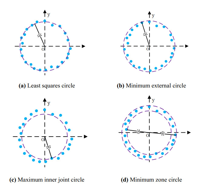
[20]	X. M. Li, Z. Y. Shi, The relationship between the minimum zone circle and the maximum inscribed circle and the minimum circumscribed circle, Precis. Eng., 33 (2009), 284–290. https://doi.org/10.1016/j.precisioneng.2008.04.005 doi: 10.1016/j.precisioneng.2008.04.005
[21]	X. Wen, Q. Xia, Y. Zhao, An effective genetic algorithm for circularity error unified evaluation, Int. J. Mach. Tools Manuf., 46 (2006), 1770–1777. https://doi.org/10.1016/j.ijmachtools.2005.11.015 doi: 10.1016/j.ijmachtools.2005.11.015
[22]	L. M. Zhu, H. Ding, Y. L. Xiong, A steepest descent algorithm for circularity evaluation, Comput. Aided Des., 35 (2003), 255–265. https://doi.org/10.1016/S0010-4485(01)00210-X doi: 10.1016/S0010-4485(01)00210-X
[23]	W. L. Yue, Y. Wu, Fast and accurate evaluation of the roundness error based on quasi-incremental algorithm, Chin. J. Mech. Eng-En., 1 (2008), 87–91. https://doi.org/10.3901/JME.2008.01.087 doi: 10.3901/JME.2008.01.087
[24]	R. Andrea, A. Michele, B. L. M. Michele, Fast genetic algorithm for roundness evaluation by the minimum zone tolerance (MZT) method, Measurement, 44 (2011), 1243–1252. https://doi.org/10.1016/j.measurement.2011.03.03101 doi: 10.1016/j.measurement.2011.03.03101
[25]	R. Calvo, E. Gómez, Accurate evaluation of functional roundness from point coordinates, Measurement, 73 (2015), 211–225. https://doi.org/ 10.1016/j.measurement.2015.04.009 doi: 10.1016/j.measurement.2015.04.009

Reader Comments

Your name:*

Email:*
© 2022 the Author(s), licensee AIMS Press. This is an open access article distributed under the terms of the Creative Commons Attribution License (http://creativecommons.org/licenses/by/4.0)