Obesity and type 2 and diabetes mellitus (T2D) are two dual epidemics whose shared genetic pathological mechanisms are still far from being fully understood. Therefore, this study is aimed at discovering key genes, molecular mechanisms, and new drug targets for obesity and T2D by analyzing the genome wide gene expression data with different computational biology approaches. In this study, the RNA-sequencing data of isolated primary human adipocytes from individuals who are lean, obese, and T2D was analyzed by an integrated framework consisting of gene expression, protein interaction network (PIN), tissue specificity, and druggability approaches. Our findings show a total of 1932 unique differentially expressed genes (DEGs) across the diabetes versus obese group comparison (p≤0.05). The PIN analysis of these 1932 DEGs identified 190 high centrality network (HCN) genes, which were annotated against 3367 GO terms and functional pathways, like response to insulin signaling, phosphorylation, lipid metabolism, glucose metabolism, etc. (p≤0.05). By applying additional PIN and topological parameters to 190 HCN genes, we further mapped 25 high confidence genes, functionally connected with diabetes and obesity traits. Interestingly, ERBB2, FN1, FYN, HSPA1A, HBA1, and ITGB1 genes were found to be tractable by small chemicals, antibodies, and/or enzyme molecules. In conclusion, our study highlights the potential of computational biology methods in correlating expression data to topological parameters, functional relationships, and druggability characteristics of the candidate genes involved in complex metabolic disorders with a common etiological basis.
Citation: Abdulhadi Ibrahim H. Bima, Ayman Zaky Elsamanoudy, Walaa F Albaqami, Zeenath Khan, Snijesh Valiya Parambath, Nuha Al-Rayes, Prabhakar Rao Kaipa, Ramu Elango, Babajan Banaganapalli, Noor A. Shaik. Integrative system biology and mathematical modeling of genetic networks identifies shared biomarkers for obesity and diabetes[J]. Mathematical Biosciences and Engineering, 2022, 19(3): 2310-2329. doi: 10.3934/mbe.2022107
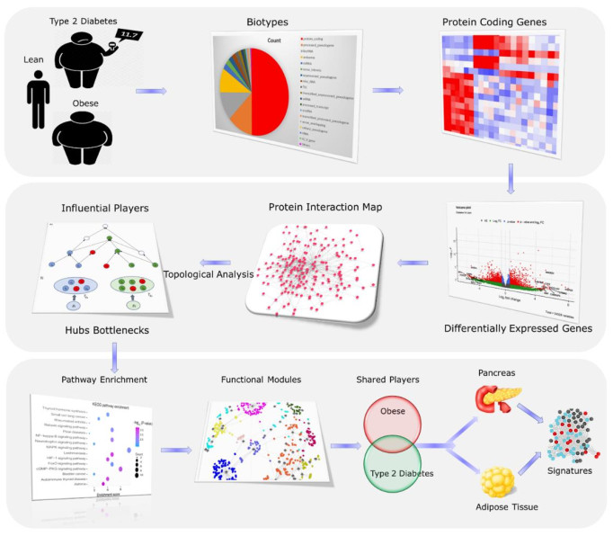
Obesity and type 2 and diabetes mellitus (T2D) are two dual epidemics whose shared genetic pathological mechanisms are still far from being fully understood. Therefore, this study is aimed at discovering key genes, molecular mechanisms, and new drug targets for obesity and T2D by analyzing the genome wide gene expression data with different computational biology approaches. In this study, the RNA-sequencing data of isolated primary human adipocytes from individuals who are lean, obese, and T2D was analyzed by an integrated framework consisting of gene expression, protein interaction network (PIN), tissue specificity, and druggability approaches. Our findings show a total of 1932 unique differentially expressed genes (DEGs) across the diabetes versus obese group comparison (p≤0.05). The PIN analysis of these 1932 DEGs identified 190 high centrality network (HCN) genes, which were annotated against 3367 GO terms and functional pathways, like response to insulin signaling, phosphorylation, lipid metabolism, glucose metabolism, etc. (p≤0.05). By applying additional PIN and topological parameters to 190 HCN genes, we further mapped 25 high confidence genes, functionally connected with diabetes and obesity traits. Interestingly, ERBB2, FN1, FYN, HSPA1A, HBA1, and ITGB1 genes were found to be tractable by small chemicals, antibodies, and/or enzyme molecules. In conclusion, our study highlights the potential of computational biology methods in correlating expression data to topological parameters, functional relationships, and druggability characteristics of the candidate genes involved in complex metabolic disorders with a common etiological basis.

| [1] |
A. S. Al-Goblan, M. A. Al-Alfi, M. Z. Khan. Mechanism linking diabetes mellitus and obesity, Diabetes Metab. Syndr. Obes., 7 (2014), 587–591. doi: 10.2147/dmso.S67400 doi: 10.2147/dmso.S67400

|
| [2] | A. A. Rao, N. M. Tayaru, H. Thota, S. B. Changalasetty, L. S. Thota, S. Gedela, Bioinformatic analysis of functional proteins involved in obesity associated with diabetes, Int. J. Biomed. Sci., 4 (2008), 70–73. |
| [3] |
P. E. Scherer, J. A. Hill, Obesity, diabetes, and cardiovascular diseases: A compendium, Circ. Res., 118 (2016), 1703–1705. doi: 10.1161/circresaha.116.308999 doi: 10.1161/circresaha.116.308999
|
| [4] |
G. R. Babu, G. V. S. Murthy, Y. Ana, P. Patel, R. Deepa, S. E. B. Neelon, et al. Association of obesity with hypertension and type 2 diabetes mellitus in India: A meta-analysis of observational studies, World J. Diabetes, 9 (2018), 40–52. doi: 10.4239/wjd.v9.i1.40 doi: 10.4239/wjd.v9.i1.40
|
| [5] |
A. Medina-Remón, R. Kirwan, R. M. Lamuela-Raventós, R. Estruch. Dietary patterns and the risk of obesity, type 2 diabetes mellitus, cardiovascular diseases, asthma, and neurodegenerative diseases, Crit. Rev. Food Sci. Nutr., 58 (2018), 262–296. doi: 10.1080/10408398.2016.1158690 doi: 10.1080/10408398.2016.1158690
|
| [6] |
G. A. Bray, Medical consequences of obesity, J. Clin. Endocrinol. Metab., 89 (2004), 2583–2589. doi: 10.1210/jc.2004-0535 doi: 10.1210/jc.2004-0535
|
| [7] |
J. S. M. Sabir, A. El Omri, B. Banaganapalli, N. Aljuaid, A. M. S. Omar, A. Altaf, et al., Unraveling the role of salt-sensitivity genes in obesity with integrated network biology and co-expression analysis, PLoS One, 15 (2020), e0228400. doi: 10.1371/journal.pone.0228400 doi: 10.1371/journal.pone.0228400
|
| [8] |
M. B. Zimering, V. Delic, B. A. Citron, Gene expression changes in a model neuron cell line exposed to autoantibodies from patients with traumatic brain injury and/or Type 2 diabetes, Mol. Neurobiol., (2021). doi: 10.1007/s12035-021-02428-4 doi: 10.1007/s12035-021-02428-4
|
| [9] |
T. O. Kilpeläinen, T. A. Lakka, D. E. Laaksonen, J. Lindström, J. G. Eriksson, T. T. Valle, et al., SNPs in PPARG associate with type 2 diabetes and interact with physical activity, Med. Sci. Sports Exerc., 40 (2008), 25–33. doi: 10.1249/mss.0b013e318159d1cd doi: 10.1249/mss.0b013e318159d1cd
|
| [10] |
J. J. Jia, X. Zhang, C. R. Ge, M. Jois, The polymorphisms of UCP2 and UCP3 genes associated with fat metabolism, obesity and diabetes, Obes. Rev., 10 (2009), 519–526. doi: 10.1111/j.1467-789X.2009.00569.x doi: 10.1111/j.1467-789X.2009.00569.x
|
| [11] |
D. Meyre, N. Bouatia-Naji, A. Tounian, C. Samson, C. Lecoeur, V. Vatin, et al., Variants of ENPP1 are associated with childhood and adult obesity and increase the risk of glucose intolerance and type 2 diabetes, Nat. Genet., 37 (2005), 863–867. doi: 10.1038/ng1604 doi: 10.1038/ng1604
|
| [12] |
T. M. Frayling, N. J. Timpson, M. N. Weedon, E. Zeggini, R. M. Freathy, C. M. Lindgren, et al., A common variant in the FTO gene is associated with body mass index and predisposes to childhood and adult obesity, Science, 316 (2007), 889–894. doi: 10.1126/science.1141634 doi: 10.1126/science.1141634
|
| [13] |
M. Hong, S. Tao, L. Zhang, L.-T. Diao, X. Huang, S. Huang, et al., RNA sequencing: New technologies and applications in cancer research, J. Hematol. Oncol., 13 (2020), 166. doi: 10.1186/s13045-020-01005-x doi: 10.1186/s13045-020-01005-x
|
| [14] |
G. Laenen, L. Thorrez, D. Börnigen, Y. Moreau, Finding the targets of a drug by integration of gene expression data with a protein interaction network, Mol. Biosyst., 9 (2013), 1676–1685. doi: 10.1039/c3mb25438k doi: 10.1039/c3mb25438k
|
| [15] |
R. Roy, L. N. Winteringham, T. Lassmann, A. R. R. Forrest. Expression levels of therapeutic targets as indicators of sensitivity to targeted therapeutics, Mol. Cancer Ther., 18 (2019), 2480–2489. doi: 10.1158/1535-7163.Mct-19-0273 doi: 10.1158/1535-7163.Mct-19-0273
|
| [16] |
R. Edgar, M. Domrachev, A. E. Lash, Gene expression omnibus: NCBI gene expression and hybridization array data repository, Nucleic Acids Res., 30 (2002), 207–210. doi: 10.1093/nar/30.1.207 doi: 10.1093/nar/30.1.207
|
| [17] |
S. W. Wingett, S. Andrews, FastQ screen: A tool for multi-genome mapping and quality control, F1000Res, 7 (2018), 1338. doi: 10.12688/f1000research.15931.2 doi: 10.12688/f1000research.15931.2
|
| [18] |
A. M. Bolger, M. Lohse, B. Usadel, Trimmomatic: A flexible trimmer for Illumina sequence data, Bioinformatics, 30 (2014), 2114–2120. doi: 10.1093/bioinformatics/btu170 doi: 10.1093/bioinformatics/btu170
|
| [19] |
A. Dobin, C. A. Davis, F. Schlesinger, J. Drenkow, C. Zaleski, S. Jha, et al., STAR: Ultrafast universal RNA-seq aligner, Bioinformatics, 29 (2013), 15–21. doi: 10.1093/bioinformatics/bts635 doi: 10.1093/bioinformatics/bts635
|
| [20] |
Y. Liao, G. K. Smyth, W. Shi, featureCounts: An efficient general purpose program for assigning sequence reads to genomic features, Bioinformatics, 30 (2014), 923–930. doi: 10.1093/bioinformatics/btt656 doi: 10.1093/bioinformatics/btt656
|
| [21] |
M. I. Love, W. Huber, S. Anders, Moderated estimation of fold change and dispersion for RNA-seq data with DESeq2, Genome Biol., 15 (2014), 550. doi: 10.1186/s13059-014-0550-8 doi: 10.1186/s13059-014-0550-8
|
| [22] | R. Kolde, pheatmap: Pretty Heatmaps. R package version 1.0. 8, in, Available, 2015. |
| [23] | K. Blighe, S. Rana, M. Lewis, EnhancedVolcano: Publication-ready volcano plots with enhanced colouring and labeling (2019), R Package Version, 1 (2018). |
| [24] |
M. H. Schaefer, J. F. Fontaine, A. Vinayagam, P. Porras, E. E. Wanker, M. A. Andrade-Navarro, HIPPIE: Integrating protein interaction networks with experiment based quality scores, PLoS One, 7 (2012), e31826. doi: 10.1371/journal.pone.0031826 doi: 10.1371/journal.pone.0031826
|
| [25] |
G. Alanis-Lobato, M. A. Andrade-Navarro, M. H. Schaefer, HIPPIE v2.0: Enhancing meaningfulness and reliability of protein-protein interaction networks, Nucleic Acids Res., 45 (2017), D408–D414. doi: 10.1093/nar/gkw985 doi: 10.1093/nar/gkw985
|
| [26] |
P. Shannon, A. Markiel, O. Ozier, N. S. Baliga, J. T. Wang, D. Ramage, et al., Cytoscape: A software environment for integrated models of biomolecular interaction networks, Genome Res., 13 (2003), 2498–2504. doi: 10.1101/gr.1239303 doi: 10.1101/gr.1239303
|
| [27] |
Y. Tang, M. Li, J. Wang, Y. Pan, F. X. Wu. CytoNCA: A cytoscape plugin for centrality analysis and evaluation of protein interaction networks, Biosystems, 127 (2015), 67–72. doi: 10.1016/j.biosystems.2014.11.005 doi: 10.1016/j.biosystems.2014.11.005
|
| [28] | S. Wasserman, K. Faust, Social network analysis: Methods and applications, (1994). |
| [29] |
S. P. Borgatti, Centrality and network flow, Social networks, 27 (2005), 55–71. doi: 10.1016/j.socnet.2004.11.008 doi: 10.1016/j.socnet.2004.11.008
|
| [30] |
L. C. Freeman, Centrality in social networks conceptual clarification, Social networks, 1 (1978), 215–239. doi: 10.1016/0378-8733(78)90021-7 doi: 10.1016/0378-8733(78)90021-7
|
| [31] | M. E. Newman, The mathematics of networks, The new palgrave encyclopedia of economics, 2 (2008), 1–12. |
| [32] |
G. George, S. Valiya Parambath, S. B. Lokappa, J. Varkey, Construction of Parkinson's disease marker-based weighted protein-protein interaction network for prioritization of co-expressed genes, Gene, 697 (2019), 67–77. doi: 10.1016/j.gene.2019.02.026 doi: 10.1016/j.gene.2019.02.026
|
| [33] |
C. Durón, Y. Pan, D. H. Gutmann, J. Hardin, A. Radunskaya, Variability of betweenness centrality and its effect on identifying essential genes, Bull. Math. Biol., 81 (2019), 3655–3673. doi: 10.1007/s11538-018-0526-z doi: 10.1007/s11538-018-0526-z
|
| [34] |
J. Chen, E. E. Bardes, B. J. Aronow, A. G. Jegga, ToppGene Suite for gene list enrichment analysis and candidate gene prioritization, Nucleic Acids Res., 37 (2009), W305–311. doi: 10.1093/nar/gkp427 doi: 10.1093/nar/gkp427
|
| [35] |
C. S. Greene, A. Krishnan, A. K. Wong, E. Ricciotti, R. A. Zelaya, D. S. Himmelstein, et al., Understanding multicellular function and disease with human tissue-specific networks, Nat. Genet., 47 (2015), 569–576. doi: 10.1038/ng.3259 doi: 10.1038/ng.3259
|
| [36] |
G. Koscielny, P. An, D. Carvalho-Silva, J. A. Cham, L. Fumis, R. Gasparyan, et al., Open Targets: A platform for therapeutic target identification and validation, Nucleic Acids Res., 45 (2017), D985–d994. doi: 10.1093/nar/gkw1055 doi: 10.1093/nar/gkw1055
|
| [37] |
C. L. Haase, A. Tybjærg-Hansen, B. G. Nordestgaard, R. Frikke-Schmidt, HDL cholesterol and risk of Type 2 diabetes: A mendelian randomization study, Diabetes, 64 (2015), 3328–3333. doi: 10.2337/db14-1603 doi: 10.2337/db14-1603
|
| [38] | M. A. Javed Shaikh, R. S. H. Singh, S. Rawat, S. Pathak, A. Mishra, et al., Role of various gene expressions in etiopathogenesis of Type 2 diabetes mellitus, Adv. Mind. Body Med., 35 (2021), 31 –39. PMID: 34237027. |
| [39] |
T. Liu, J. Liu, L. Hao, Network pharmacological study and molecular docking analysis of qiweitangping in treating diabetic coronary heart disease, Evid. Based Complement. Alternat. Med., 2021 (2021), 9925556. doi: 10.1155/2021/9925556 doi: 10.1155/2021/9925556
|
| [40] |
N. N. Sahly, B. Banaganapalli, A. N. Sahly, A. H. Aligiraigri, K. K. Nasser, T. Shinawi, et al., Molecular differential analysis of uterine leiomyomas and leiomyosarcomas through weighted gene network and pathway tracing approaches, Syst. Biol. Reprod. Med., 67 (2021), 209–220. doi: 10.1080/19396368.2021.1876179 doi: 10.1080/19396368.2021.1876179
|
| [41] |
B. Banaganapalli, N. Al-Rayes, Z. A. Awan, F. A. Alsulaimany, A. S. Alamri, R. Elango, et al., Multilevel systems biology analysis of lung transcriptomics data identifies key miRNAs and potential miRNA target genes for SARS-CoV-2 infection, Comput. Biol. Med., 135 (2021), 104570. doi: 10.1016/j.compbiomed.2021.104570 doi: 10.1016/j.compbiomed.2021.104570
|
| [42] |
A. Mujalli, B. Banaganapalli, N. M. Alrayes, N. A. Shaik, R. Elango, J. Y. Al-Aama, Myocardial infarction biomarker discovery with integrated gene expression, pathways and biological networks analysis, Genomics, 112 (2020), 5072–5085. doi: 10.1016/j.ygeno.2020.09.004 doi: 10.1016/j.ygeno.2020.09.004
|
| [43] |
T. Ideker, R. Nussinov, Network approaches and applications in biology, PLoS Comput. Biol., 13 (2017), e1005771–e1005771. doi: 10.1371/journal.pcbi.1005771 doi: 10.1371/journal.pcbi.1005771
|
| [44] |
D. O. Holland, B. H. Shapiro, P. Xue, M. E. Johnson, Protein-protein binding selectivity and network topology constrain global and local properties of interface binding networks, Sci. Rep., 7 (2017), 5631. doi: 10.1038/s41598-017-05686-2 doi: 10.1038/s41598-017-05686-2
|
| [45] |
Y. Gao, X. Chang, J. Xia, S. Sun, Z. Mu, X. Liu, Identification of HCC-related genes based on differential partial correlation network, Front Genet, 12 (2021), 672117. doi: 10.3389/fgene.2021.672117 doi: 10.3389/fgene.2021.672117
|
| [46] |
C. Liu, L. Lu, Q. Kong, Y. Li, H. Wu, W. Yang, et al., Developing discriminate model and comparative analysis of differentially expressed genes and pathways for bloodstream samples of diabetes mellitus type 2, BMC Bioinform., 15 Suppl 17 (2014), S5. doi: 10.1186/1471-2105-15-s17-s5 doi: 10.1186/1471-2105-15-s17-s5
|
| [47] |
G. Prashanth, B. Vastrad, A. Tengli, C. Vastrad, I. Kotturshetti, Investigation of candidate genes and mechanisms underlying obesity associated type 2 diabetes mellitus using bioinformatics analysis and screening of small drug molecules, BMC Endocr. Disord., 21 (2021), 80. doi: 10.1186/s12902-021-00718-5 doi: 10.1186/s12902-021-00718-5
|
| [48] |
X. Yao, J. Yan, K. Liu, S. Kim, K. Nho, S. L. Risacher, et al., Tissue-specific network-based genome wide study of amygdala imaging phenotypes to identify functional interaction modules, Bioinformatics, 33 (2017), 3250–3257. doi: 10.1093/bioinformatics/btx344 doi: 10.1093/bioinformatics/btx344
|
| [49] | R. L. J. van Meijel, E. E. Blaak, G. H. Goossens, Chapter 1 - Adipose tissue metabolism and inflammation in obesity, in: R. A. Johnston, B. T. Suratt (Eds.), Mechanisms and Manifestations of Obesity in Lung Disease, Academic Press, 2019, pp. 1–22. |
| [50] |
C. Fotis, A. Antoranz, D. Hatziavramidis, T. Sakellaropoulos, L. G. Alexopoulos, Network-based technologies for early drug discovery, Drug Discovery Today, 23 (2018), 626–635. doi: 10.1016/j.drudis.2017.12.001 doi: 10.1016/j.drudis.2017.12.001
|
| [51] |
J. M. Fernandez-Real, J. A. Menendez, J. M. Moreno-Navarrete, M. Blüher, A. Vazquez-Martin, M. J. Vázquez, et al., Extracellular fatty acid synthase: A possible surrogate biomarker of insulin resistance, Diabetes, 59 (2010), 1506–1511. doi: 10.2337/db09-1756 doi: 10.2337/db09-1756
|
| [52] |
A. Ray, Tumor-linked HER2 expression: Association with obesity and lipid-related microenvironment, Horm. Mol. Biol. Clin. Investig., 32 (2017). doi: 10.1515/hmbci-2017-0020 doi: 10.1515/hmbci-2017-0020
|
| [53] |
F. J. Ruiz-Ojeda, A. Méndez-Gutiérrez, C. M. Aguilera, J. Plaza-Díaz, Extracellular matrix remodeling of adipose tissue in obesity and metabolic diseases, Int. J. Mol. Sci., 20 (2019). doi: 10.3390/ijms20194888 doi: 10.3390/ijms20194888
|
| [54] |
P. Järgen, A. Dietrich, A. W. Herling, H. P. Hammes, P. Wohlfar, The role of insulin resistance in experimental diabetic retinopathy-Genetic and molecular aspects, PLoS One, 12 (2017), e0178658. doi: 10.1371/journal.pone.0178658 doi: 10.1371/journal.pone.0178658
|
| [55] |
M. C. Tse, X. Liu, S. Yang, K. Ye, C. B. Chan, Fyn regulates adipogenesis by promoting PIKE-A/STAT5a interaction, Mol. Cell. Biol., 33 (2013), 1797–1808. doi: 10.1128/mcb.01410-12 doi: 10.1128/mcb.01410-12
|
| [56] |
C. C. Bastie, H. Zong, J. Xu, B. Busa, S. Judex, I. J. Kurland, et al., Integrative metabolic regulation of peripheral tissue fatty acid oxidation by the SRC kinase family member Fyn, Cell Metab., 5 (2007), 371–381. doi: 10.1016/j.cmet.2007.04.005 doi: 10.1016/j.cmet.2007.04.005
|
| [57] |
E. Yamada, J. E. Pessin, I. J. Kurland, G. J. Schwartz, C. C. Bastie, Fyn-dependent regulation of energy expenditure and body weight is mediated by tyrosine phosphorylation of LKB1, Cell Metab., 11 (2010), 113–124. doi: 10.1016/j.cmet.2009.12.010 doi: 10.1016/j.cmet.2009.12.010
|
| [58] | C. C. Bastie, H. H. Zong, J. Xu, S. Judex, I. J. Kurland, J. E. Pessin, Fyn kinase deficiency increases peripheral tissue insulin sensitivity by improving fatty acid oxidation and lipolysis, Diabetes, 56 (2007), A60. |
| [59] |
J. Rodrigues-Krause, M. Krause, C. O'Hagan, G. De Vito, C. Boreham, C. Murphy, et al., Divergence of intracellular and extracellular HSP72 in type 2 diabetes: Does fat matter?, Cell Stress Chaperones, 17 (2012), 293–302. doi: 10.1007/s12192-011-0319-x doi: 10.1007/s12192-011-0319-x
|
| [60] |
P. L. Hooper, G. Balogh, E. Rivas, K. Kavanagh, L. Vigh, The importance of the cellular stress response in the pathogenesis and treatment of type 2 diabetes, Cell Stress Chaperones, 19 (2014), 447–464. doi: 10.1007/s12192-014-0493-8 doi: 10.1007/s12192-014-0493-8
|
| [61] |
E. Chang, M. Varghese, K. Singer, Gender and sex differences in adipose tissue, Curr. Diab. Rep., 18 (2018), 69. doi: 10.1007/s11892-018-1031-3 doi: 10.1007/s11892-018-1031-3
|


Figures(8) / Tables(4)

Abdulhadi Ibrahim H. Bima, Ayman Zaky Elsamanoudy, Walaa F Albaqami, Zeenath Khan, Snijesh Valiya Parambath, Nuha Al-Rayes, Prabhakar Rao Kaipa, Ramu Elango, Babajan Banaganapalli, Noor A. Shaik. Integrative system biology and mathematical modeling of genetic networks identifies shared biomarkers for obesity and diabetes[J]. Mathematical Biosciences and Engineering, 2022, 19(3): 2310-2329. doi: 10.3934/mbe.2022107


 DownLoad: