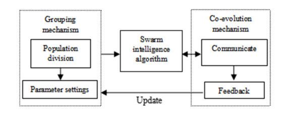
The balance between exploration and exploitation is critical to the performance of a Meta-heuristic optimization method. At different stages, a proper tradeoff between exploration and exploitation can drive the search process towards better performance. This paper develops a multi-objective grasshopper optimization algorithm (MOGOA) with a new proposed framework called the Multi-group and Co-evolution Framework which can archive a fine balance between exploration and exploitation. For the purpose, a grouping mechanism and a co-evolution mechanism are designed and integrated into the framework for ameliorating the convergence and the diversity of multi-objective optimization solutions and keeping the exploration and exploitation of swarm intelligence algorithm in balance. The grouping mechanism is employed to improve the diversity of search agents for increasing coverage of search space. The co-evolution mechanism is used to improve the convergence to the true Pareto optimal front by the interaction of search agents. Quantitative and qualitative outcomes prove that the framework prominently ameliorate the convergence accuracy and convergence speed of MOGOA. The performance of the presented algorithm has been benchmarked by several standard test functions, such as CEC2009, ZDT and DTLZ. The diversity and convergence of the obtained multi-objective optimization solutions are quantitatively and qualitatively compared with the original MOGOA by using two performance indicators (GD and IGD). The results on test suits show that the diversity and convergence of the obtained solutions are significantly improved. On several test functions, some statistical indicators are more than doubled. The validity of the results has been verified by the Wilcoxon rank-sum test.
Citation: Chao Wang, Jian Li, Haidi Rao, Aiwen Chen, Jun Jiao, Nengfeng Zou, Lichuan Gu. Multi-objective grasshopper optimization algorithm based on multi-group and co-evolution[J]. Mathematical Biosciences and Engineering, 2021, 18(3): 2527-2561. doi: 10.3934/mbe.2021129
The balance between exploration and exploitation is critical to the performance of a Meta-heuristic optimization method. At different stages, a proper tradeoff between exploration and exploitation can drive the search process towards better performance. This paper develops a multi-objective grasshopper optimization algorithm (MOGOA) with a new proposed framework called the Multi-group and Co-evolution Framework which can archive a fine balance between exploration and exploitation. For the purpose, a grouping mechanism and a co-evolution mechanism are designed and integrated into the framework for ameliorating the convergence and the diversity of multi-objective optimization solutions and keeping the exploration and exploitation of swarm intelligence algorithm in balance. The grouping mechanism is employed to improve the diversity of search agents for increasing coverage of search space. The co-evolution mechanism is used to improve the convergence to the true Pareto optimal front by the interaction of search agents. Quantitative and qualitative outcomes prove that the framework prominently ameliorate the convergence accuracy and convergence speed of MOGOA. The performance of the presented algorithm has been benchmarked by several standard test functions, such as CEC2009, ZDT and DTLZ. The diversity and convergence of the obtained multi-objective optimization solutions are quantitatively and qualitatively compared with the original MOGOA by using two performance indicators (GD and IGD). The results on test suits show that the diversity and convergence of the obtained solutions are significantly improved. On several test functions, some statistical indicators are more than doubled. The validity of the results has been verified by the Wilcoxon rank-sum test.

| [1] |
S. Saremi, S. Mirjalili, A. Lewis, Grasshopper Optimisation Algorithm: Theory and application, Adv. Eng. Software, 105 (2017), 30–47. doi: 10.1016/j.advengsoft.2017.01.004

|
| [2] |
M. Laszczyk, P. B. Myszkowski, Improved selection in evolutionary multi–objective optimization of Multi–Skill Resource–Constrained Project Scheduling Problem, Inf. Sci., 481 (2019), 412–431. doi: 10.1016/j.ins.2019.01.002
|
| [3] |
G. Eichfelder, J. Niebling, S. Rocktäschel, An algorithmic approach to multi-objective optimization with decision uncertainty, J. Global Optim., 77 (2020), 3–25. doi: 10.1007/s10898-019-00815-9
|
| [4] | D. Simon, Evolutionary Optimization Algorithms, John Wiley & Sons, Hoboken, NJ, 2013. |
| [5] | K. Deb, Multi-objective optimization, Search Methodologies, Search Methodol., 2014 (2014), 403–449. |
| [6] | T. Eftimov, P. Koroec, Deep Statistical Comparison for Multi-Objective Stochastic Optimization Algorithms, Swarm Evol. Comput., 61 (2020), 100837. |
| [7] | G. G. Wang, S. Deb, Z. Cui, Monarch butterfly optimization, Neural Comput. Appl., 31 (2015), 1995–2014. |
| [8] |
S. Li, H. Chen, M. Wang, A. A. Heidari, S. Mirjalili, Slime mould algorithm: A new method for stochastic optimization, Future Gener. Comput. Syst., 111 (2020), 300–323. doi: 10.1016/j.future.2020.03.055
|
| [9] |
G. G. Wang, Moth search algorithm: a bio-inspired metaheuristic algorithm for global optimization problems, Memetic Comput., 10 (2018), 151–164 doi: 10.1007/s12293-016-0212-3
|
| [10] |
A. A. Heidari, S. Mirjalili, H. Faris, I. Aljarah, M. Mafarja, H. Chen, Harris hawks optimization: Algorithm and applications, Future Gener. Comput. Syst., 97 (2019), 849–872. doi: 10.1016/j.future.2019.02.028
|
| [11] |
L. Lin, M. Gen, Auto-tuning strategy for evolutionary algorithms: balancing between exploration and exploitation, Soft Comput., 13 (2009), 157–168. doi: 10.1007/s00500-008-0303-2
|
| [12] | X. S. Yang, Nature-Inspired Metaheuristic Algorithms, Luniver Press, 2010. |
| [13] |
I. Boussad, J. Lepagnot, P. Siarry, A survey on optimization metaheuristics, Inf. Sci., 237 (2013), 82–117. doi: 10.1016/j.ins.2013.02.041
|
| [14] |
S. Z. Mirjalili, S. Mirjalili, S. Saremi, H. Faris, I. Aljarah, Grasshopper optimization algorithm for multi-objective optimization problems, Appl. Intell., 48 (2018), 805–820. doi: 10.1007/s10489-018-1251-x
|
| [15] | K. Deb, S. Mittal, D. K. Saxena, E. D. Goodman, Embedding a Repair Operator in Evolutionary Single and Multi-Objective Algorithms-An Exploitation-Exploration Perspective, Evolutionary Multi-Criterion Optimization (EMO-2021), 2021. |
| [16] |
D. Li, W. Guo, A. Lerch, Y. Li, L. Wang, Q. Wu, An adaptive particle swarm optimizer with decoupled exploration and exploitation for large scale optimization, Swarm Evol. Comput., 60 (2021), 100789. doi: 10.1016/j.swevo.2020.100789
|
| [17] |
M. Abdel-Basset, R. Mohamed, M. Abouhawwash, Balanced multi-objective optimization algorithm using improvement based reference points approach, Swarm Evol. Comput., 60 (2021), 100791. doi: 10.1016/j.swevo.2020.100791
|
| [18] |
H. Zhang, J. Sun, T. Liu, K. Zhang, Q. Zhang, Balancing Exploration and Exploitation in Multi-objective Evolutionary Optimization, Inf. Sci., 497 (2019), 129–148. doi: 10.1016/j.ins.2019.05.046
|
| [19] |
P. Koroec, T. Eftimov, Insights into Exploration and Exploitation Power of Optimization Algorithm Using DSC Tool, Mathematics, 8 (2020), 1474–1484. doi: 10.3390/math8091474
|
| [20] | S. H. Liu, M. Mernik, B. R. Bryant, To explore or to exploit: An entropy-driven approach for evolutionary algorithms, Int. J. Knowl. Based Intell. Eng. Syst., 13 (2009), 185–206. |
| [21] | J. J. Liang, P. N. Suganthan, Dynamic Multi-Swarm Particle Swarm Optimizer with a Novel Constraint-Handling Mechanism, IEEE International Conference on Evolutionary Computation, IEEE, 2006. |
| [22] |
X. Wu, S. Zhang, W. Xiao, Y. Yin, The Exploration/Exploitation Tradeoff in Whale Optimization Algorithm, IEEE Access, 7 (2019), 125919–125928. doi: 10.1109/ACCESS.2019.2938857
|
| [23] |
T. Jiang, C. Zhang, H. Zhu, J. Gu, G. Deng, Energy-efficient scheduling for a job shop using an improved whale optimization algorithm, Mathematics, 6 (2018), 220–236. doi: 10.3390/math6110220
|
| [24] |
J. Too, A. R. Abdullah, N. M. Saad, A New Co-Evolution Binary Particle Swarm Optimization with Multiple Inertia Weight Strategy for Feature Selection, Informatics, 6 (2019), 21–34. doi: 10.3390/informatics6020021
|
| [25] |
L. Abualigah, A. Diabat, A comprehensive survey of the Grasshopper optimization algorithm: results, variants, and applications, Neural Comput. Appl., 32 (2020), 15533–15556. doi: 10.1007/s00521-020-04789-8
|
| [26] | R. A. Ibrahim, A. A. Ewees, D. Oliva, M. A. Elaziz, S. Lu, Improved salp swarm algorithm based on particle swarm optimization for feature selection, J. Ambient Intell. Humanized Comput., 10 (2018), 3155–3169. |
| [27] |
K. Li, S. Kwong, Q. Zhang, K. Deb, Interrelationship-Based Selection for Decomposition Multiobjective Optimization, IEEE Trans. Cybern., 45 (2015), 2076–2088. doi: 10.1109/TCYB.2014.2365354
|
| [28] | S. W. Jiang, Z. H. Cai, J. Zhang, Y. S. Ong, Multiobjective optimization bydecomposition with Pareto-adaptive weight vectors, Seventh International Conference on Natural Computation, IEEE, 2011. |
| [29] |
S. Shahbeig, A. Rahideh, M. S. Helfroush, K. Kazemi, Gene selection from large-scale gene expression data based on fuzzy interactive multi-objective binary optimization for medical diagnosis, Biocybern. Biomed. Eng., 38 (2018), 313–328. doi: 10.1016/j.bbe.2018.02.002
|
| [30] | S. Kim, I. J. Jeong, Interactive Multi-Objective Optimization Using Mobile Application: Application to Multi-Objective Linear Assignment Problem, Proceedings of the 2019 Asia Pacific Information Technology Conference, 2019. |
| [31] | M. Sakawa, Fuzzy Multiobjective Optimization, in Multicriteria Decision Aid and Artificial Intelligence, John Wiley & Sons, Ltd, 2013,235–271. |
| [32] | Y. Tian, S. Yang, X. Zhang, An Evolutionary Multi-objective Optimization Based Fuzzy Method for Overlapping Community Detection, IEEE Trans. Fuzzy Syst., 28 (2019), 2841–2855. |
| [33] | N. Piegay, D. Breysse, Multi-Objective Optimization and Decision Aid for Spread Footing Design in Uncertain Environment, in Geotechnical Safety and Risk V, IOS Press, 2015,419–424. |
| [34] |
E. D. Comanita, C. Ghinea, R. M. Hlihor, I. M. Simion, C. Smaranda, L. Favier, et al., Challenges and opportunities in green plastics: an assessment using the electre decision-aid method, Environ. Eng. Manage. J., 14 (2015), 689–702. doi: 10.30638/eemj.2015.077
|
| [35] |
J. Zhou, X. Yao, L. Gao, C. Hu, An indicator and adaptive region division based evolutionary algorithm for many-objective optimization, Appl. Soft Comput., 99 (2021), 106872. doi: 10.1016/j.asoc.2020.106872
|
| [36] |
H. Zhang, Q. Hui, Many objective cooperative bat searching algorithm, Appl. Soft Comput., 77 (2019), 412–437. doi: 10.1016/j.asoc.2019.01.033
|
| [37] |
I. H. Osman, G. Laporte, Metaheuristics: A bibliography, Ann. Oper. Res., 63 (1996), 511–623. doi: 10.1007/BF02125421
|
| [38] |
S. Santander-Jiménez, M. A. Vega-Rodríguez, L. Sousa, A multiobjective adaptive approach for the inference of evolutionary relationships in protein-based scenarios, Inf. Sci., 485 (2019), 281–300. doi: 10.1016/j.ins.2019.02.020
|
| [39] |
B. Yazid, B. Sadek, C. Djamal, Evolutionary Metaheuristics to Solve Multiobjective Assignment Problem in Telecommunication Network: Multiobjective Assignment Problem, Int. J. Appl. Metaheuristic Comput., 11 (2020), 56–76. doi: 10.4018/IJAMC.2020040103
|
| [40] | Á. Rubio-Largo, L. Vanneschi, M. Castelli, M. A. Vega-Rodríguez, Multiobjective Meta-heuristic to Design RNA Sequences, IEEE Trans. Evol. Comput., 23 (2018), 156–169. |
| [41] |
S. Safarzadeh, S. Shadrokh, A. Salehian, A heuristic scheduling method for the pipe-spool fabrication process, J. Ambient Intell. Humanized Comput., 9 (2018), 1901–1918. doi: 10.1007/s12652-018-0737-z
|
| [42] |
S. Safarzadeh, H. Koosha, Solving an extended multi-row facility layout problem with fuzzy clearances using GA, Appl. Soft Comput., 61 (2017), 819–831. doi: 10.1016/j.asoc.2017.09.003
|
| [43] | C. M. Rahman, T. A. Rashid, A new evolutionary algorithm: Learner performance based behavior algorithm, Egypt. Inf. J., (2020), forthcoming. |
| [44] | C. M. Rahman, T. A. Rashid, Dragonfly Algorithm and its Applications in Applied Science Survey, Comput. Intell. Neurosci., 2019 (2019), 9293617. |
| [45] | A. M. Ahmed, T. A. Rashid, S. M. Saeed, Cat Swarm Optimization Algorithm: A Survey and Performance Evaluation, Comput. Intell. Neurosci., 2020 (2020), 20. |
| [46] | B. A. Hassan, T. A. Rashid, Operational Framework for Recent Advances in Backtracking Search Optimisation Algorithm: A Systematic Review and Performance Evaluation, Appl. Math. Comput., 370 (2019), 124919. |
| [47] |
A. S. Shamsaldin, T. A. Rashid, R. A. Al-Rashid, N. K. Al-Salihi, M. Mohammadi, Donkey and Smuggler Optimization Algorithm: A Collaborative Working Approach to Path Finding, J. Comput. Design Eng., 6 (2019), 562–583. doi: 10.1016/j.jcde.2019.04.004
|
| [48] |
J. M. Abdullah, T. Rashid, Fitness Dependent Optimizer: Inspired by the Bee Swarming Reproductive Process, IEEE Access, 7 (2019), 43473–43486. doi: 10.1109/ACCESS.2019.2907012
|
| [49] |
D. A. Muhammed, S. A. M. Saeed, T. A. Rashid, Improved Fitness-Dependent Optimizer Algorithm, IEEE Access, 8 (2020), 19074–19088. doi: 10.1109/ACCESS.2020.2968064
|
| [50] |
M. A. Montes, T. Stutzle, M. Birattari, M. Dorigo, Frankenstein's PSO: A Composite Particle Swarm Optimization Algorithm, IEEE Trans. Evol. Comput., 13 (2009), 1120–1132. doi: 10.1109/TEVC.2009.2021465
|
| [51] |
Q. T. Vien, T. A. Le, X. S. Yang, T. Q. Duong, Enhancing Security of MME Handover via Fractional Programming and Firefly Algorithm, IEEE Trans. Commun., 67 (2019), 6206–6220. doi: 10.1109/TCOMM.2019.2920353
|
| [52] |
G. J. Ibrahim, T. A. Rashid, M. O. Akinsolu, An energy efficient service composition mechanism using a hybrid meta-heuristic algorithm in a mobile cloud environment, J. Parallel Distrib. Comput., 143 (2020), 77–87. doi: 10.1016/j.jpdc.2020.05.002
|
| [53] |
H. Mohammed, T. A. Rashid, A Novel Hybrid GWO with WOA for Global Numerical Optimization and Solving Pressure Vessel Design, Neural Comput. Appl., 32 (2020), 14701–14718. doi: 10.1007/s00521-020-04823-9
|
| [54] | H. M. Mohammed, S. U. Umar, T. A. Rashid, A Systematic and Meta-analysis Survey of Whale Optimization Algorithm, Comput. Intell. Neurosci., 2019 (2019), 8718571. |
| [55] |
P. Sharma, A. Gupta, A. Aggarwal, D. Gupta, A. Khanna, A. E. Hassanien, The health of things for classification of protein structure using improved grey wolf optimization, J. Supercomput., 76 (2020), 1226–1241. doi: 10.1007/s11227-018-2639-4
|
| [56] |
H. Zhang, S. Su, A hybrid multi-agent Coordination Optimization Algorithm, Swarm Evol. Comput., 51 (2019), 100603. doi: 10.1016/j.swevo.2019.100603
|
| [57] |
H. Jia, Y. Li, C. Lang, X. Peng, K. Sun, J. Li, Hybrid grasshopper optimization algorithm and differential evolution for global optimization, J. Intell. Fuzzy Syst., 37 (2019), 6899–6910. doi: 10.3233/JIFS-190782
|
| [58] |
Q. Lin, Q. Zhu, P. Huang, J. Chen, Z. Ming, J. Yu, A novel hybrid multi-objective immune algorithm with adaptive differential evolution, Comput. Oper. Res., 62 (2015), 95–111. doi: 10.1016/j.cor.2015.04.003
|
| [59] |
S. Arora, P. Anand, Chaotic grasshopper optimization algorithm for global optimization, Neural Comput. Appl., 31 (2019), 4385–4405. doi: 10.1007/s00521-018-3343-2
|
| [60] | Z. Elmi, M. Ö. Efe, Multi-objective grasshopper optimization algorithm for robot path planning in static environments, 2018 IEEE International Conference on Industrial Technology, 2018. |
| [61] | S. Rangasamy, Y. Kuppusami, A Novel Nature-Inspired Improved Grasshopper Optimization-Tuned Dual-Input Controller for Enhancing Stability of Interconnected Systems, J. Circuits Syst. Comput., 2020 (2020), 21501346. |
| [62] |
X. Zhang, Q. Miao, H. Zhang, L. Wang, A parameter-adaptive VMD method based on grasshopper optimization algorithm to analyze vibration signals from rotating machinery, Mech. Syst. Signal Process., 108 (2018), 58–72. doi: 10.1016/j.ymssp.2017.11.029
|
| [63] | S. Dwivedi, M. Vardhan, S. Tripathi, Building an efficient intrusion detection system using grasshopper optimization algorithm for anomaly detection, Cluster Comput., 2021 (2021), 1–20. |
| [64] | Y. Li, L. Gu, Grasshopper optimization algorithm based on curve adaptive and simulated annealing, Appl. Res. Comput., 36 (2019), 3637–3643. |
| [65] | R. Yaghobzadeh, S. R. Kamel, M. Asgari, H. Saadatmand, A Binary Grasshopper Optimization Algorithm for Feature Selection, Int. J. Eng. Res. Technol., 9 (2020), 533–540. |
| [66] |
S. Dwivedi, M. Vardhan, S. Tripathi, An Effect of Chaos Grasshopper Optimization Algorithm for Protection of Network Infrastructure, Comput. Networks, 176 (2020), 107251. doi: 10.1016/j.comnet.2020.107251
|
| [67] | R. V. Rao, Application of TLBO and ETLBO Algorithms on Complex Composite Test Functions, Teaching Learning Based Optimization Algorithm, 2016. |
| [68] |
E. Zitzler, K. Deb, L. Thiele, Comparison of multiobjective evolutionary algorithms: Empirical results, Evol. Comput., 8 (2000), 173–195. doi: 10.1162/106365600568202
|
| [69] | K. Deb, L. Thiele, M. Laumanns, E. Zitzler, Scalable multi-objective optimization test problems, Proceedings of the 2002 congress on evolutionary computation, 2002. |
| [70] | Q. Zhang, A. Zhou, S. Zhao, P. N. Suganthan, W. Liu, S. Tiwari, Multiobjective optimization test instances for the CEC 2009 special session and competition, University of Essex, Colchester, UK and Nanyang Technological University, Rep. CES, 487 (2008), 2008. |
Figures(8) / Tables(16)

Chao Wang, Jian Li, Haidi Rao, Aiwen Chen, Jun Jiao, Nengfeng Zou, Lichuan Gu. Multi-objective grasshopper optimization algorithm based on multi-group and co-evolution[J]. Mathematical Biosciences and Engineering, 2021, 18(3): 2527-2561. doi: 10.3934/mbe.2021129


 DownLoad: