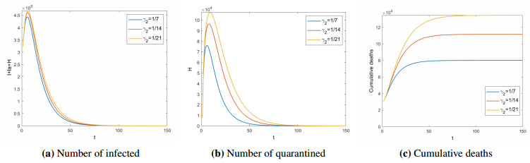
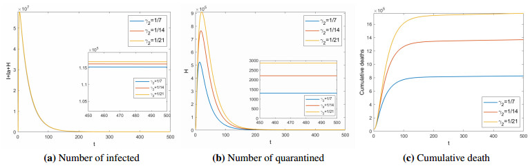
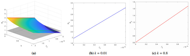
In this paper, we present an SEII$ { _\rm a} $HR epidemic model to study the influence of recessive infection and isolation in the spread of COVID-19. We first prove that the infection-free equilibrium is globally asymptotically stable with condition $ R_0 < 1 $ and the positive equilibrium is uniformly persistent when the condition $ R_0 > 1 $. By using the COVID-19 data in India, we then give numerical simulations to illustrate our results and carry out some sensitivity analysis. We know that asymptomatic infections will affect the spread of the disease when the quarantine rate is within the range of [0.3519, 0.5411]. Furthermore, isolating people with symptoms is important to control and eliminate the disease.
Citation: Rong Yuan, Yangjun Ma, Congcong Shen, Jinqing Zhao, Xiaofeng Luo, Maoxing Liu. Global dynamics of COVID-19 epidemic model with recessive infection and isolation[J]. Mathematical Biosciences and Engineering, 2021, 18(2): 1833-1844. doi: 10.3934/mbe.2021095
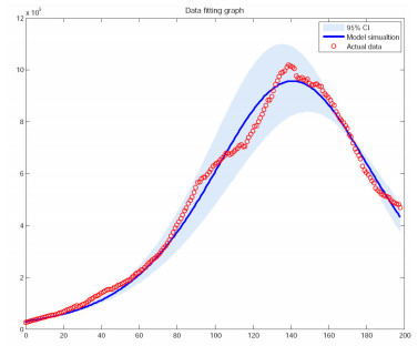
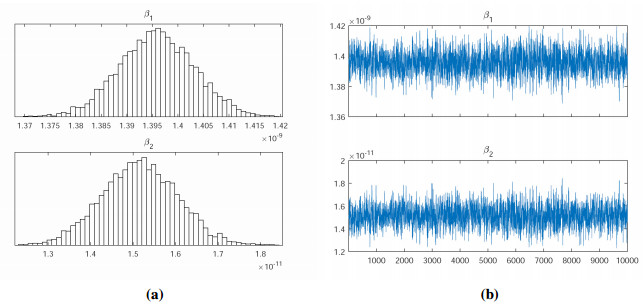
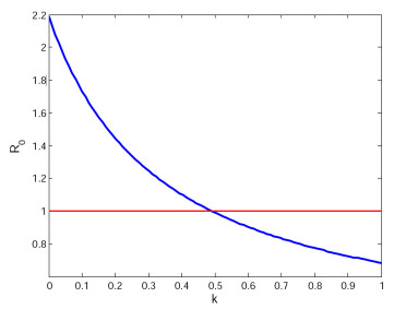
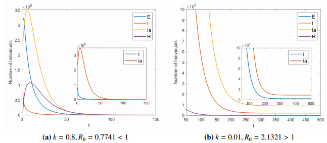
In this paper, we present an SEII$ { _\rm a} $HR epidemic model to study the influence of recessive infection and isolation in the spread of COVID-19. We first prove that the infection-free equilibrium is globally asymptotically stable with condition $ R_0 < 1 $ and the positive equilibrium is uniformly persistent when the condition $ R_0 > 1 $. By using the COVID-19 data in India, we then give numerical simulations to illustrate our results and carry out some sensitivity analysis. We know that asymptomatic infections will affect the spread of the disease when the quarantine rate is within the range of [0.3519, 0.5411]. Furthermore, isolating people with symptoms is important to control and eliminate the disease.

| [1] | WHO, Coronavirus disease (COVID-19) Pandemic, 2020. Available at https://www.who.int/emergencies/diseases/novel-coronavirus-2019. |
| [2] |
J. Jiao, Z. Liu, S. Cai, Dynamics of an SEIR model with infectivity in incubation period and homestead-isolation on the susceptible, Appl. Math. Lett., 107 (2020), 106442. doi: 10.1016/j.aml.2020.106442

|
| [3] |
M. Li, G. Sun, J. Zhang, Y. Zhao, Z. Jin, Analysis of COVID-19 transmission in Shanxi Province with discrete time imported cases, Math. Biosci. Eng., 17 (2020), 3710–3720. doi: 10.3934/mbe.2020208
|
| [4] |
Z. Xu, L. Shi, Y. Wang, J. Huang, L. Zhang, C. Liu, et al., Pathological findings of COVID-19 associated with acute respiratory distress syndrome, Lancet Respir. Med., 8 (2020), 420–422. doi: 10.1016/S2213-2600(20)30076-X
|
| [5] |
B. Cao, Y. Wang, D. Wen, W. Liu, J. Wang, G. Fan, et al., A Trial of Lopinavir-Ritonavir in Adults Hospitalized with Severe Covid-19, New Engl. J. Med., 382 (2020), 1787–1799. doi: 10.1056/NEJMoa2001282
|
| [6] |
C. Wang, R. Pan, X. Wan, Y. Tan, L. Xu, C. Ho, et al., Immediate Psychological Responses and Associated Factors during the Initial Stage of the 2019 Coronavirus Disease (COVID-19) Epidemic among the General Population in China, Int. J. Env. Res. Pub. He., 17 (2020), 1729. doi: 10.3390/ijerph17051729
|
| [7] |
J. Hellewell, S. Abbott, A. Gimma, N. I. Bosse, C. I. Jarvis, T. W. Russell, et al., Feasibility of controlling COVID-19 outbreaks by isolation of cases and contacts, Lancet Glob. Health, 8 (2020), 488–496. doi: 10.1016/S2214-109X(20)30074-7
|
| [8] |
S. He, Y. Peng, K. Sun, SEIR modeling of the COVID-19 and its dynamics, Nonlinear Dynam., 101 (2020), 1667–1680. doi: 10.1007/s11071-020-05743-y
|
| [9] |
C. Eastin, T. Eastin, Clinical Characteristics of Coronavirus Disease 2019 in China, J. Emerg. Med., 58 (2020), 711–712. doi: 10.1016/j.jemermed.2020.04.004
|
| [10] |
W. O. Kermack, A. G. McKendrick, A Contribution to the Mathematical Theory of Epidemics, Proc. R. Soc. Lond. A, 115 (1927), 700–721. doi: 10.1098/rspa.1927.0118
|
| [11] |
J. Zhang, Z. Jin, G. Sun, S. Ruan, Modeling seasonal rabies epidemics in China, B. Math. Biol., 74 (2012), 1226–1251. doi: 10.1007/s11538-012-9720-6
|
| [12] |
J. Zhang, Z. Jin, G. Sun, T. Zhou, S. Ruan, Analysis of rabies in China: transmission dynamics and control, PLoS One, 6 (2011), e20891. doi: 10.1371/journal.pone.0020891
|
| [13] |
D. Z. Gao, S. Ruan, A multipatch malaria model with logistic growth populations, SIAM. J. Appl. Math., 72 (2012), 819–841. doi: 10.1137/110850761
|
| [14] |
G. Q. Sun, J. H. Xie, S. H. Huang, Z. Jin, M. T. Li, L. Liu, Transmission dynamics of cholera: mathematical modeling and control strategies, Commun. Nonlinear Sci. Numer. Simul., 45 (2017), 235–244. doi: 10.1016/j.cnsns.2016.10.007
|
| [15] |
J. Zhang, G. Q. Sun, X. D. Sun, Q. Hou, M. T. Li, B. X. Huang, et al., Prediction and control of brucellosis transmission of dairy cattle in Zhejiang Province, China, PLoS One, 9 (2014), e108592. doi: 10.1371/journal.pone.0108592
|
| [16] |
Y. Ma, M. Liu, Q. Hou, J. Zhao, Modeling seasonal HFMD with the recessive infection in Shandong, China, Math. Biosci. Eng., 10 (2013), 1159–1171. doi: 10.3934/mbe.2013.10.1159
|
| [17] |
A. Bouchnita, A. Jebrane, A multi-scale model quantifies the impact of limited movement of the population and mandatory wearing of face masks in containing the COVID-19 epidemic in Morocco, Mathe. Model. Nat. Pheno., 15 (2020), 50. doi: 10.1051/mmnp/2020040
|
| [18] |
X. Chang, M. Liu, Z. Jin, J. Wang, Studying on the impact of media coverage on the spread of COVID-19 in Hubei Province, China, Math. Biosci. Eng., 17 (2020), 3147–3159. doi: 10.3934/mbe.2020178
|
| [19] |
X. Bardina, M. Ferrante, C. Rovira, A stochastic epidemic model of COVID-19 disease, AIMS Math., 5(2020), 7661–7677. doi: 10.3934/math.2020490
|
| [20] | Z. Zhang, A. Zeb, S. Hussain, E. Alzahrani, Dynamics of COVID-19 mathematical model with stochastic perturbation, Adv. Differ. Equations, 2020 (2020). |
| [21] |
A. J. Kucharski, T. W. Russell, C. Diamond, Y. Liu, J. Edmunds, S. Funk, et al., Early dynamics of transmission and control of COVID-19: a mathematical modelling study, Lancet Infect. Dis., 20 (2020), 553–558. doi: 10.1016/S1473-3099(20)30144-4
|
| [22] |
Z. Liu, P. Magal, O. Seydi, G. Webb, Understanding Unreported Cases in the COVID-19 Epidemic Outbreak in Wuhan, China, and the Importance of Major Public Health Interventions, Biology, 9 (2020), 50. doi: 10.3390/biology9030050
|
| [23] |
H. S. Badr, H. Du, M. Marshall, E. Dong, M. M. Squire, L. M. Gardner, Association between mobility patterns and COVID-19 transmission in the USA: a mathematical modelling study, Lancet Infect. Dis., 20 (2020), 1247–1254. doi: 10.1016/S1473-3099(20)30553-3
|
| [24] | Y. Liu, A. A. Gayle, A. Wilder-Smith, J. Rocklov, The reproductive number of COVID-19 is higher compared to SARS coronavirus, J. Travel Med., 27 (2020), 1–4. |
| [25] | O. Diekmann, J. A. P. Heesterbeek, J. A. J. Metz, On the definition and the computation of the basic reproduction ratio $R_0$ in models for infectious diseases in heterogeneous populations, J. Math. Biol., 28 (1990), 365–382. |
| [26] |
P. van den Driessche, J. Watmough, Reproduction numbers and sub-threshold endemic equilibria for compartmental models of disease transmission, Math. Biosci., 180 (2002), 29–48. doi: 10.1016/S0025-5564(02)00108-6
|
| [27] |
H. I. Freedman, S. Ruan, M. Tang, Uinform persistence and flows near a closed positicve invariant set, J. Dyn. Differ. Equations, 6 (1994), 583–600. doi: 10.1007/BF02218848
|
| [28] | X. Zhao, Dynamical System in Population Biology, Springer, 2003. |
| [29] | India Population, https://countrymeters.info/en/India. |
| [30] | Mary Van Beusekom, Study: Many asymptomatic COVID-19 cases undetected, https://www.cidrap.umn.edu/news-perspective/2020/04/study-many-asymptomatic-covid-19-cases-undetected. |
| [31] | K. Sarkar, S. Khajanchi, Modeling and forecasting of the COVID-19 pandemic in India, preprint, arXiv: 2005.07071. |
| [32] | B. Tang, N. L. Bragazzi, Q. Li, S. Tang, Y. Xiao, J. Wu, An updated estimation of the risk of transmission of the novel coronavirus (2019-nCov), Infect. Dis. Model., 5 (2020), 248–255. |
| [33] | Ministry of health and welfare, government of India, https://www.governement.in/, 2020. |
Figures(7) / Tables(2)

Rong Yuan, Yangjun Ma, Congcong Shen, Jinqing Zhao, Xiaofeng Luo, Maoxing Liu. Global dynamics of COVID-19 epidemic model with recessive infection and isolation[J]. Mathematical Biosciences and Engineering, 2021, 18(2): 1833-1844. doi: 10.3934/mbe.2021095


 DownLoad: