On the determination of first-mode stress intensity factors and T-stress in a continuous functionally graded beam using digital image correlation method

Ahmed M. Abood; Haider Khazal; Abdulkareem F. Hassan; Ahmed M. Abood; Haider Khazal; Abdulkareem F. Hassan

doi:10.3934/matersci.2022004

AIMS Materials Science

2022, Volume 9, Issue 1: 56-70. doi: 10.3934/matersci.2022004

Previous Article Next Article

Research article Topical Sections

On the determination of first-mode stress intensity factors and T-stress in a continuous functionally graded beam using digital image correlation method

Department of mechanical engineering, College of engineering, University of Basrah, Basrah, ‎Iraq

Received: 09 September 2021 Revised: 28 October 2021 Accepted: 02 November 2021 Published: 28 December 2021

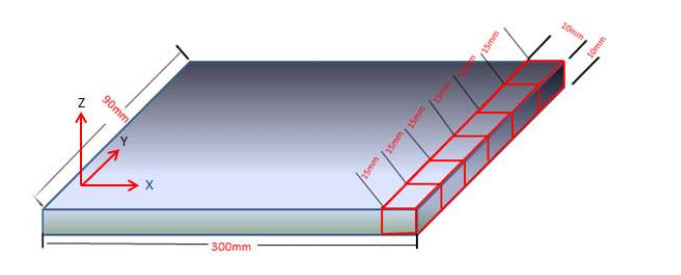
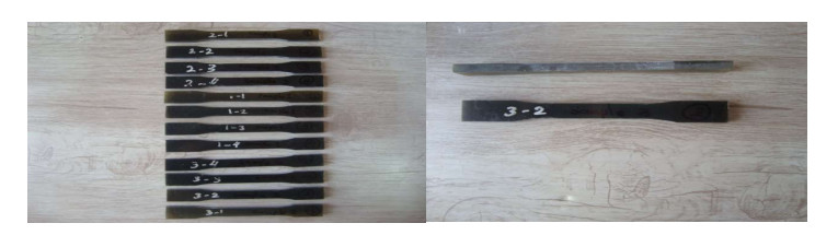
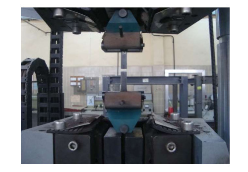
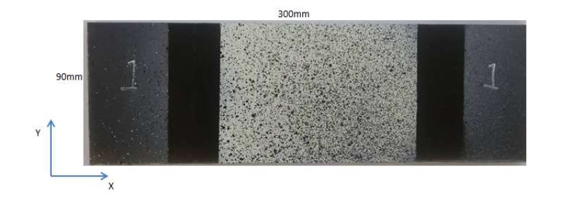
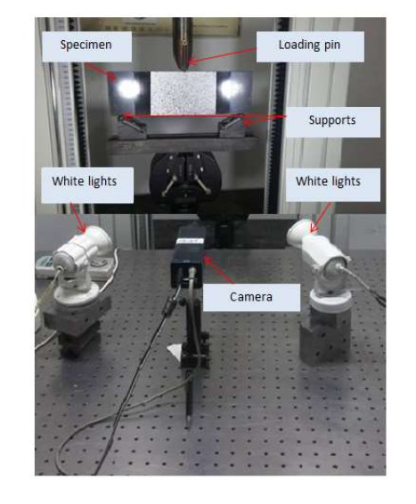
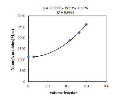
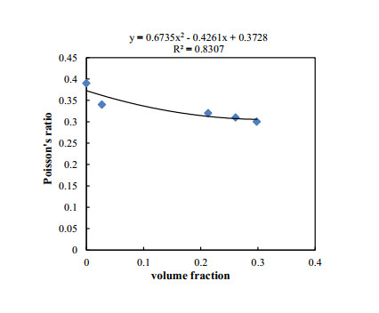
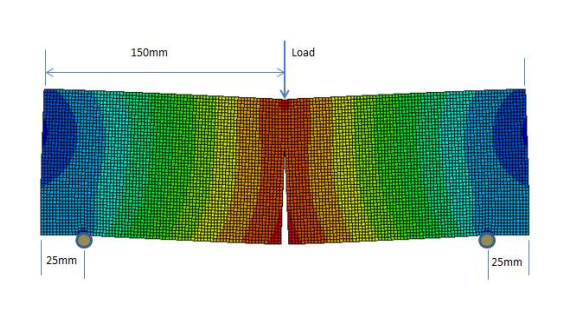
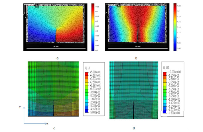
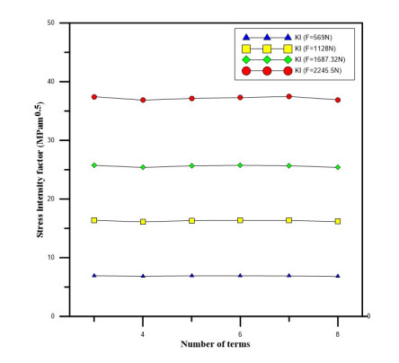
In this study, fracture parameters of epoxy/glass functionally graded composite were determined experimentally using the digital image correlation (DIC) method. A functionally graded material (FGM) with continuous variation in elastic properties was manufactured by gravity casting in vertical template. A 30% volume fraction of glass spheres was dispersed in a low viscosity resin. A single edge crack specimen was examined in a three-point bending test under mode Ⅰ loading with cracks along the gradient tendency of the material properties. The mechanical properties of FGM were calculated according to ASTM D638. The DIC technique was adopted to obtain the deformation region around the crack tip. William's series was employed to calculate stress intensity factor and T-stress. The experimental results then verified by solving the FE model using ABAQUS program. The comparison between DIC and numerical results illustrated a largely acceptable achievement.
- continuous FGM,
- Digital Image Correlation (DIC),
- three-point bending beam,
- T-stress,
- Stress Intensity Factors (SIFs)
Citation: Ahmed M. Abood, Haider Khazal, Abdulkareem F. Hassan. On the determination of first-mode stress intensity factors and T-stress in a continuous functionally graded beam using digital image correlation method[J]. AIMS Materials Science, 2022, 9(1): 56-70. doi: 10.3934/matersci.2022004

Related Papers:

Abstract

In this study, fracture parameters of epoxy/glass functionally graded composite were determined experimentally using the digital image correlation (DIC) method. A functionally graded material (FGM) with continuous variation in elastic properties was manufactured by gravity casting in vertical template. A 30% volume fraction of glass spheres was dispersed in a low viscosity resin. A single edge crack specimen was examined in a three-point bending test under mode Ⅰ loading with cracks along the gradient tendency of the material properties. The mechanical properties of FGM were calculated according to ASTM D638. The DIC technique was adopted to obtain the deformation region around the crack tip. William's series was employed to calculate stress intensity factor and T-stress. The experimental results then verified by solving the FE model using ABAQUS program. The comparison between DIC and numerical results illustrated a largely acceptable achievement.

References

[1]	Pei G, Asaro RJ (1997) Cracks in functionally graded materials. Int J Solids Struct 34: 1–17. https://doi.org/10.1016/0020-7683(95)00289-8 doi: 10.1016/0020-7683(95)00289-8
[2]	Miyamoto Y, Kaysser WA, Rabin BH, et al. (2013) Functionally Graded Materials: Design, Processing and Applications, New York: Springer Science & Business Media.
[3]	Farouq W, Khazal H, Hassan AKF (2019) Fracture analysis of functionally graded material using digital image correlation technique and extended element-free Galerkin method. Opt Laser Eng 121: 307–322. https://doi.org/10.1016/j.optlaseng.2019.04.021 doi: 10.1016/j.optlaseng.2019.04.021
[4]	Jin ZH, Batra RC (1996) Some basic fracture mechanics concepts in functionally graded materials. J Mech Phys Solids 44: 1221–1235. https://doi.org/10.1016/0022-5096(96)00041-5 doi: 10.1016/0022-5096(96)00041-5
[5]	Dolbow JE, Gosz M (2002) On the computation of mixed-mode stress intensity factors in functionally graded materials. Int J Solids Struct 39: 2557–2574. https://doi.org/10.1016/S0020-7683(02)00114-2 doi: 10.1016/S0020-7683(02)00114-2
[6]	Butcher RJ, Rousseau CE, Tippur HV (1998) A functionally graded particulate composite: preparation, measurements and failure analysis. Acta Mater 47: 259–268. https://doi.org/10.1016/S1359-6454(98)00305-X doi: 10.1016/S1359-6454(98)00305-X
[7]	Rousseau CE, Tippur HV (2002) Evaluation of crack tip fields and stress intensity factors in functionally graded elastic materials: cracks parallel to elastic gradient. Int J Fracture 114: 87–112. https://doi.org/10.1023/A:1014889628080 doi: 10.1023/A:1014889628080
[8]	Rousseau CE, Tippur HV (2000) Compositionally graded materials with cracks normal to the elastic gradient. Acta Mater 48: 4021–4033. https://doi.org/10.1016/S1359-6454(00)00202-0 doi: 10.1016/S1359-6454(00)00202-0
[9]	Rousseau CE, Tippur HV (2002) Influence of elastic variations on crack initiation in functionally graded glass-filled epoxy. Eng Fract Mech 69: 1679–1693. https://doi.org/10.1016/S0013-7944(02)00056-5 doi: 10.1016/S0013-7944(02)00056-5
[10]	Jain N, Rousseau CE, Shukla A (2004) Crack-tip stress fields in functionally graded materials with linearly varying properties. Theor Appl Fract Mec 42: 155–170. https://doi.org/10.1016/j.tafmec.2004.08.005 doi: 10.1016/j.tafmec.2004.08.005
[11]	Nakamura T, Wang T, Sampath S (2000) Determination of properties of graded materials by inverse analysis and instrumented indentation. Acta Mater 48: 4293–4306. https://doi.org/10.1016/S1359-6454(00)00217-2 doi: 10.1016/S1359-6454(00)00217-2
[12]	Kim JH, Paulino GH (2002) Finite element evaluation of mixed mode stress intensity factors in functionally graded materials. Int J Numer Methods Eng 53: 1903–1935. https://doi.org/10.1002/nme.364 doi: 10.1002/nme.364
[13]	Kirugulige MS, Tippur HV (2006) Mixed-mode dynamic crack growth in functionally graded glass-filled epoxy. Exp Mech 46: 269–281. https://doi.org/10.1007/s11340-006-5863-4 doi: 10.1007/s11340-006-5863-4
[14]	Khazal H, Hassan AKF, Farouq W, et al. (2019) Computation of fracture parameters in stepwise functionally graded materials using digital image correlation technique. Mater Perform Charac 8: 344–354. https://doi.org/10.1520/MPC20180175 doi: 10.1520/MPC20180175
[15]	Yao XF, Xiong TC, Xu W, et al. (2006) Experimental investigations on deformation and fracture behavior of glass sphere filled epoxy functionally graded materials. Appl Compos Mater 13: 407–420. https://doi.org/10.1007/s10443-006-9026-7 doi: 10.1007/s10443-006-9026-7
[16]	Jin X, Wu L, Guo L, et al. (2009) Experimental investigation of the mixed-mode crack propagation in ZrO₂/NiCr functionally graded materials. Eng Fract Mech 76: 1800–1810. https://doi.org/10.1016/j.engfracmech.2009.04.003 doi: 10.1016/j.engfracmech.2009.04.003
[17]	Yates JR, Zanganeh M, Tai YH (2010) Quantifying crack tip displacement fields with DIC. Eng Fract Mech 77: 2063–2076. https://doi.org/10.1016/j.engfracmech.2010.03.025 doi: 10.1016/j.engfracmech.2010.03.025
[18]	Jones SA, Tomlinson RA (2015) Investigating mixed-mode (I/II) fracture in epoxies using digital image correlation: Composite GIIc performance from resin measurements. Eng Fract Mech 149: 368–374. https://doi.org/10.1016/j.engfracmech.2015.08.041 doi: 10.1016/j.engfracmech.2015.08.041
[19]	Khazal H, Bayesteh H, Mohammadi S, et al. (2016) An extended element free Galerkin method for fracture analysis of functionally graded materials. Mech Adv Mater Struc 23: 513–528. https://doi.org/10.1080/15376494.2014.984093 doi: 10.1080/15376494.2014.984093
[20]	Khazal H, Saleh NA (2019) XEFGM for crack propagation analysis of functionally graded materials under mixed-mode and non-proportional loading. Mech Adv Mater Struc 26: 975–983. https://doi.org/10.1080/15376494.2018.1432786 doi: 10.1080/15376494.2018.1432786
[21]	Mousa S, Abd-Elhady AA, Abu-Sinna A, et al. (2019) Mixed mode crack growth in functionally graded material under three-point bending. Pro Struc Int 17: 284–291. https://doi.org/10.1016/j.prostr.2019.08.038 doi: 10.1016/j.prostr.2019.08.038
[22]	Fatima NS, Rowlands RE (2020) SIF determination in finite double-edge cracked orthotropic composite using J-integral and digital image correlation. Eng Fract Mech 235: 107099. https://doi.org/10.1016/j.engfracmech.2020.107099 doi: 10.1016/j.engfracmech.2020.107099
[23]	Quanjin M, Rejab MRM, Halim Q, et al. (2020) Experimental investigation of the tensile test using digital image correlation (DIC) method. Mater Today 27: 757–763. https://doi.org/10.1016/j.matpr.2019.12.072 doi: 10.1016/j.matpr.2019.12.072
[24]	Abshirini M, Dehnavi MY, Beni MA, et al. (2014) Interaction of two parallel U-notches with tip cracks in PMMA plates under tension using digital image correlation. Theor Appl Fract Mec 70: 75–82. https://doi.org/10.1016/j.tafmec.2014.02.001 doi: 10.1016/j.tafmec.2014.02.001
[25]	Golewski GL (2021) Evaluation of fracture processes under shear with the use of DIC technique in fly ash concrete and accurate measurement of crack path lengths with the use of a new crack tip tracking method. Measurement 181: 109632. https://doi.org/10.1016/j.measurement.2021.109632 doi: 10.1016/j.measurement.2021.109632
[26]	Golewski GL (2021) Validation of the favorable quantity of fly ash in concrete and analysis of crack propagation and its length–Using the crack tip tracking (CTT) method–In the fracture toughness examinations under Mode II, through digital image correlation. Constr Build Mater 296: 122362. https://doi.org/10.1016/j.conbuildmat.2021.122362 doi: 10.1016/j.conbuildmat.2021.122362
[27]	Golewski GL, Gil DM (2021) Studies of fracture toughness in concretes containing fly ash and silica fume in the first 28 days of curing. Mater 14: 319. https://doi.org/10.3390/ma14020319 doi: 10.3390/ma14020319
[28]	Eshraghi I, Dehnavi MRY, Soltani N (2014) Effect of subset parameters selection on the estimation of mode-I stress intensity factor in a cracked PMMA specimen using digital image correlation. Polym Test 37: 193–200. https://doi.org/10.1016/j.polymertesting.2014.05.017 doi: 10.1016/j.polymertesting.2014.05.017

Reader Comments

Your name:*

Email:*
© 2022 the Author(s), licensee AIMS Press. This is an open access article distributed under the terms of the Creative Commons Attribution License (http://creativecommons.org/licenses/by/4.0)