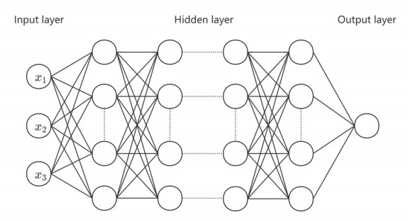
Having accurate knowledge on CO2 solubility in reservoir liquids plays a pivotal role in geoenergy harvest and carbon capture, utilization, and storage (CCUS) applications. Data-driven works leveraging artificial neural networks (ANN) have presented a promising tool for forecasting CO2 solubility. In this paper, an ANN model was developed based on hundreds of documented data to predict CO2 solubility in both pure water and saline solutions across a broad spectrum of temperatures, pressures, and salinities in reference to underground formation conditions. Multilayer perceptron (MLP) models were constructed for each system, and their prediction results were rigorously validated against the the literature data. The research results indicate that the ANN model is suitable for predicting the solubility of carbon dioxide under different conditions, with root mean square errors (RMSE) of 0.00108 and 0.00036 for water and brine, and a coefficient of determination (R2) of 0.99424 and 0.99612, which indicates robust prediction capacities. It was observed from the ANN model that the saline water case could not be properly expanded to predict the CO2 solubility in pure water, underscoring the distinct dissolution mechanisms in polar mixtures. It is expected that this study could provide a valuable reference and offer novel insights to the prediction of CO2 solubility in complex fluid systems.
Citation: Shuo Yang, Dong Wang, Zeguang Dong, Yingge Li, Dongxing Du. ANN prediction of the CO2 solubility in water and brine under reservoir conditions[J]. AIMS Geosciences, 2025, 11(1): 201-227. doi: 10.3934/geosci.2025009
Having accurate knowledge on CO2 solubility in reservoir liquids plays a pivotal role in geoenergy harvest and carbon capture, utilization, and storage (CCUS) applications. Data-driven works leveraging artificial neural networks (ANN) have presented a promising tool for forecasting CO2 solubility. In this paper, an ANN model was developed based on hundreds of documented data to predict CO2 solubility in both pure water and saline solutions across a broad spectrum of temperatures, pressures, and salinities in reference to underground formation conditions. Multilayer perceptron (MLP) models were constructed for each system, and their prediction results were rigorously validated against the the literature data. The research results indicate that the ANN model is suitable for predicting the solubility of carbon dioxide under different conditions, with root mean square errors (RMSE) of 0.00108 and 0.00036 for water and brine, and a coefficient of determination (R2) of 0.99424 and 0.99612, which indicates robust prediction capacities. It was observed from the ANN model that the saline water case could not be properly expanded to predict the CO2 solubility in pure water, underscoring the distinct dissolution mechanisms in polar mixtures. It is expected that this study could provide a valuable reference and offer novel insights to the prediction of CO2 solubility in complex fluid systems.

| [1] | Rogelj J, Den Elzen M, Höhne N, et al. (2016) Paris Agreement climate proposals need a boost to keep warming well below 2℃. Nature: 631–639. https://doi.org/10.1038/nature18307 |
| [2] | Du D, Sun S, Zhang N, et al. (2015) Pressure distribution measurements for CO2 foam flow in porous media. J Porous Media: 1119–1126. https://doi.org/10.1615/JPorMedia.2015012151 |
| [3] |
Du D, Zhang N, Li Y, et al. (2017) Parametric studies on foam displacement behavior in a layered heterogeneous porous media based on the stochastic population balance model. J Nat Gas Sci Eng 48: 1–12. https://doi.org/10.1016/j.jngse.2017.08.035 doi: 10.1016/j.jngse.2017.08.035

|
| [4] |
Du D, Zhang D, Li Y, et al. (2019) Numerical investigations on the inlet and outlet behavior of foam flow process in porous media using stochastic bubble population balance model. J Pet Sci Eng 176:537–553. https://doi.org/10.1016/j.petrol.2019.01.073 doi: 10.1016/j.petrol.2019.01.073
|
| [5] |
Du D, Zhang X, Yu K, et al. (2020) Parameter Screening Study for Optimizing the Static Properties of Nanoparticle-Stabilized CO2 Foam Based on Orthogonal Experimental Design. ACS Omega 5: 4014–4023. https://doi.org/10.1021/acsomega.9b03543 doi: 10.1021/acsomega.9b03543
|
| [6] |
Du D, Zhao D, Li Y, et al. (2021) Parameter calibration of the stochastic bubble population balance model for predicting NP-stabilized foam flow characteristics in porous media. Colloids Surf A 614: 126180. https://doi.org/10.1016/j.colsurfa.2021.126180 doi: 10.1016/j.colsurfa.2021.126180
|
| [7] |
Li Y, Zhao D, Du D (2022) Computational study on the three phase displacement characteristics of foam fluids in porous media. J Pet Sci Eng 215: 110732. https://doi.org/10.1016/j.petrol.2022.110732 doi: 10.1016/j.petrol.2022.110732
|
| [8] |
Mutailipu M, Song Y, Yao Q, et al. (2024) Solubility and interfacial tension models for CO2–brine systems under CO2 geological storage conditions. Fuel 357: 129712. https://doi.org/10.1016/j.fuel.2023.129712 doi: 10.1016/j.fuel.2023.129712
|
| [9] |
Du D, Zhang X, Wan C, et al. (2021) Determination of the effective thermal conductivity of the porous media based on digital rock physics. Geothermics 97: 102267. https://doi.org/10.1016/j.geothermics.2021.102267 doi: 10.1016/j.geothermics.2021.102267
|
| [10] |
Eyitayo S, Arbad N, Okere C, et al. (2025) Advancing geological storage of carbon dioxide (CO2) with emerging technologies for climate change mitigation. Int J Environ Sci Technol 22: 5023–5056. https://doi.org/10.1007/s13762-024-06074-w doi: 10.1007/s13762-024-06074-w
|
| [11] | Liu Y, Hu T, Rui Z, et al. (2023). An Integrated Framework for Geothermal Energy Storage with CO2 Sequestration and Utilization. Engineering: 121–130. https://doi.org/10.1016/j.eng.2022.12.010 |
| [12] | Wu Y, Li P (2020) The potential of coupled carbon storage and geothermal extraction in a CO2-enhanced geothermal system: a review. Geotherm Energy 8. https://doi.org/10.1186/s40517-020-00173-w |
| [13] |
Xu Z, Zhao H, Fan L, et al. (2024) A literature review of using supercritical CO2 for geothermal energy extraction: Potential, methods, challenges, and perspectives. Renew Energ Focus 51: 100637. https://doi.org/10.1016/j.ref.2024.100637 doi: 10.1016/j.ref.2024.100637
|
| [14] |
Cui P, Liu Z, Cui X, et al. (2023) Impact of water on miscibility characteristics of the CO2/n-hexadecane system using the pendant drop shape analysis method. Arabian J Chem 16: 105038. https://doi.org/10.1016/j.arabjc.2023.105038 doi: 10.1016/j.arabjc.2023.105038
|
| [15] |
Liu Z, Yan S, Zang H, et al. (2023) Quantization of the water presence effect on the diffusion coefficients of the CO2/oil system with the dynamic pendant drop volume analysis technique. Chem Eng Sci 281: 119142. https://doi.org/10.1016/j.ces.2023.119142 doi: 10.1016/j.ces.2023.119142
|
| [16] | Hu J, Duan Z, Zhu C, et al. (2007) PVTx properties of the CO2-H2O and CO2-H2O-NaCl systems below 647 K: Assessment of experimental data and thermodynamic models. Chemical Geology: 249–267. https://doi.org/10.1016/j.chemgeo.2006.11.011 |
| [17] | Ruth LA, Squires AM, Graff RA, et al. (1991) Desulfurization of Fuels With Calcined Dolomite. 1. Introduction and First Kinetic Results. Chem Soc Diu Fuel Chem 30: 67. |
| [18] | Schmidt C, Bodnar RJ (2000) Synthetic fluid inclusions: XVI. PVTX properties in the system H2O-NaCl-CO2 at elevated temperatures, pressures, and salinites. Geochim Cosmochim Acta 64: 3853–3869. https://doi.org/10.1016/S0016-7037(00)00471-3 |
| [19] |
Wang X, Cui X, Wang F, et al. (2021) Miscibility characteristics of the CO2/n-hexadecane system with presence of water component based on the phase equilibrium calculation on the interface region. Colloids Surf A 629: 127463. https://doi.org/10.1016/j.colsurfa.2021.127463 doi: 10.1016/j.colsurfa.2021.127463
|
| [20] | Valtz A, Chapoy A, Coquelet C, et al. (2004) Vapour-liquid equilibria in the carbon dioxide-water system, measurement and modelling from 278.2 to 318.2 K. Fluid Phase Equilib 226: 333–344. https://doi.org/10.1016/j.fluid.2004.10.013 |
| [21] |
Carvalho PJ, Pereira LMC, Gonçalves NPF, et al. (2015) Carbon dioxide solubility in aqueous solutions of NaCl: Measurements and modeling with electrolyte equations of state. Fluid Phase Equilib 388: 100–106. https://doi.org/10.1016/j.fluid.2014.12.043 doi: 10.1016/j.fluid.2014.12.043
|
| [22] | Guo H, Chen Y, Hu Q, et al. (2014) Quantitative Raman spectroscopic investigation of geo-fluids high-pressure phase equilibria: Part I. Accurate calibration and determination of CO2 solubility in water from 273.15 to 573.15K and from 10 to 120MPa. Fluid Phase Equilib 382: 70–79. https://doi.org/10.1016/j.fluid.2014.08.032 |
| [23] |
Talebian SH, Masoudi R, Tan IM, et al. (2014) Foam assisted CO2-EOR: A review of concept, challenges, and future prospects. J Pet Sci Eng 120: 202–215. https://doi.org/10.1016/j.petrol.2014.05.013 doi: 10.1016/j.petrol.2014.05.013
|
| [24] | Zhao H, Lvov SN (2016) Phase behavior of the CO2-H2O system at temperatures of 273-623 K and pressures of 0.1-200 MPa using Peng-Robinson-Stryjek-Vera equation of state with a modified Wong-Sandler mixing rule: An extension to the CO2-CH4-H2O system. Fluid Phase Equilib 417: 96–108. https://doi.org/10.1016/j.fluid.2016.02.027 |
| [25] |
Cui X, Zheng L, Liu Z, et al. (2022). Determination of the Minimum Miscibility Pressure of the CO2/oil system based on quantification of the oil droplet volume reduction behavior. Colloids Surf A 653: 130058. https://doi.org/10.1016/j.colsurfa.2022.130058 doi: 10.1016/j.colsurfa.2022.130058
|
| [26] |
Peridas G, Mordick Schmidt B (2021) The role of carbon capture and storage in the race to carbon neutrality. Electr J 34: 106996. https://doi.org/10.1016/j.tej.2021.106996 doi: 10.1016/j.tej.2021.106996
|
| [27] | Zhaoa H, Fedkin MV, Dilmore RM, et al. (2015) Carbon dioxide solubility in aqueous solutions of sodium chloride at geological conditions: Experimental results at 323.15,373.15, and 423.15K and 150bar and modeling up to 573.15K and 2000bar. Geochim Cosmochim Acta 149: 165–189. https://doi.org/10.1016/j.gca.2014.11.004 |
| [28] |
Duan Z, Sun R, Zhu C, et al. (2006) An improved model for the calculation of CO2 solubility in aqueous solutions containing Na+, K+, Ca2+, Mg2+, Cl-, and SO42-. Mar Chem 98: 131–139. https://doi.org/10.1016/j.marchem.2005.09.001 doi: 10.1016/j.marchem.2005.09.001
|
| [29] | Spycher N, Pruess K, Ennis-King J (2003) CO2-H2O mixtures in the geological sequestration of CO2. I. Assessment and calculation of mutual solubilities from 12 to 100 ℃ and up to 600 bar. Geochim Cosmochim Acta 67: 3015–3031. https://doi.org/10.1016/S0016-7037(03)00273-4 |
| [30] |
Liu Z, Cui P, Cui X, et al. (2022) Prediction of CO2 solubility in NaCl brine under geological conditions with an improved binary interaction parameter in the Søreide-Whitson model. Geothermics 105: 102544. https://doi.org/10.1016/j.geothermics.2022.102544 doi: 10.1016/j.geothermics.2022.102544
|
| [31] | Schmidhuber J (2015) Deep Learning in neural networks: An overview. Neural Networks: 85–117. https://doi.org/10.1016/j.neunet.2014.09.003 |
| [32] |
Lecun Y, Bengio Y, Hinton G (2015) Deep learning. Nature 521: 436–444. https://doi.org/10.1038/nature14539 doi: 10.1038/nature14539
|
| [33] |
Vanneschi L, Castelli M (2018) Multilayer perceptrons. Encycl Bioinf Comput Biol 1: 612–620. https://doi.org/10.1016/B978-0-12-809633-8.20339-7 doi: 10.1016/B978-0-12-809633-8.20339-7
|
| [34] | Rumelhart DE, Hinton GE, Williams RJ (2019) Learning Representations by Back-Propagating Errors. Cognitive Modeling: 213–222. https://doi.org/10.7551/mitpress/1888.003.0013 |
| [35] |
Goel A, Goel AK, Kumar A (2023) The role of artificial neural network and machine learning in utilizing spatial information. Spat Inf Res 31: 275–285. https://doi.org/10.1007/s41324-022-00494-x doi: 10.1007/s41324-022-00494-x
|
| [36] | Kim H (2022) Deep Learning. In: Artificial Intelligence for 6G, 22: 247–303. https://doi.org/10.1007/978-3-030-95041-5_6 |
| [37] |
Madani SA, Mohammadi MR, Atashrouz S, et al. (2021) Modeling of nitrogen solubility in normal alkanes using machine learning methods compared with cubic and PC-SAFT equations of state. Sci Rep 11: 24403. https://doi.org/10.1038/s41598-021-03643-8 doi: 10.1038/s41598-021-03643-8
|
| [38] |
Mohammadi MR, Hadavimoghaddam F, Pourmahdi M, et al. (2021) Modeling hydrogen solubility in hydrocarbons using extreme gradient boosting and equations of state. Sci Rep 11: 17911. https://doi.org/10.1038/s41598-021-97131-8 doi: 10.1038/s41598-021-97131-8
|
| [39] | Nakhaei-Kohani R, Taslimi-Renani E, Hadavimoghaddam F, et al. (2022) Modeling solubility of CO2–N2 gas mixtures in aqueous electrolyte systems using artificial intelligence techniques and equations of state. Sci Rep 12: 3625. https://doi.org/10.1038/s41598-022-07393-z |
| [40] |
Mahmoudzadeh A, Amiri-Ramsheh B, Atashrouz S, et al. (2024). Modeling CO2 solubility in water using gradient boosting and light gradient boosting machine. Sci Rep 14: 13511. https://doi.org/10.1038/s41598-024-63159-9 doi: 10.1038/s41598-024-63159-9
|
| [41] |
Bamberger A, Sieder G, Maurer G (2004) High-pressure phase equilibrium of the ternary system carbon dioxide + water + acetic acid at temperatures from 313 to 353 K. J Supercrit Fluids 32: 15–25. https://doi.org/10.1016/j.supflu.2003.12.014 doi: 10.1016/j.supflu.2003.12.014
|
| [42] |
Chapoy A, Mohammadi AH, Chareton A, et al. (2004) Measurement and Modeling of Gas Solubility and Literature Review of the Properties for the Carbon Dioxide-Water System. Ind Eng Chem Res 43: 1794–1802. https://doi.org/10.1021/ie034232t doi: 10.1021/ie034232t
|
| [43] |
Liu Y, Hou M, Yang G, et al. (2011) Solubility of CO2 in aqueous solutions of NaCl, KCl, CaCl 2 and their mixed salts at different temperatures and pressures. J Supercrit Fluids 56: 125–129. https://doi.org/10.1016/j.supflu.2010.12.003 doi: 10.1016/j.supflu.2010.12.003
|
| [44] |
Chabab S, Théveneau P, Corvisier J, et al. (2019) Thermodynamic study of the CO2 – H2O – NaCl system: Measurements of CO2 solubility and modeling of phase equilibria using Soreide and Whitson, electrolyte CPA and SIT models. Int J Greenhouse Gas Control 91: 102825. https://doi.org/10.1016/j.ijggc.2019.102825 doi: 10.1016/j.ijggc.2019.102825
|
| [45] | Guo H, Huang Y, Chen Y, et al. (2016) Quantitative Raman Spectroscopic Measurements of CO2 Solubility in NaCl Solution from (273.15 to 473.15) K at p = (10.0, 20.0, 30.0, and 40.0) MPa. J Chem Eng Data 61: 466–474. https://doi.org/10.1021/acs.jced.5b00651 |
| [46] |
Yan W, Huang S, Stenby EH (2011) Measurement and modeling of CO2 solubility in NaCl brine and CO2-saturated NaCl brine density. Int J Greenhouse Gas Control 5: 1460–1477. https://doi.org/10.1016/j.ijggc.2011.08.004 doi: 10.1016/j.ijggc.2011.08.004
|
| [47] |
Longe PO, Danso DK, Gyamfi G, et al. (2024). Predicting CO2 and H2 Solubility in Pure Water and Various Aqueous Systems: Implication for CO2–EOR, Carbon Capture and Sequestration, Natural Hydrogen Production and Underground Hydrogen Storage. Energies 17: 5723. https://doi.org/10.3390/en17225723 doi: 10.3390/en17225723
|
| [48] |
Ng CSW, Djema H, Nait Amar M, et al. (2022) Modeling interfacial tension of the hydrogen-brine system using robust machine learning techniques: Implication for underground hydrogen storage. Int J Hydrogen Energy 47: 39595–39605. https://doi.org/10.1016/j.ijhydene.2022.09.120 doi: 10.1016/j.ijhydene.2022.09.120
|
| [49] |
Di M, Sun R, Geng L, et al. (2021) An accurate model to calculate CO2 solubility in pure water and in seawater at hydrate–liquid water two‐phase equilibrium. Minerals 11: 393. https://doi.org/10.3390/min11040393 doi: 10.3390/min11040393
|
| [50] | Zhang XQ, Yao CJ, Zhou YR, et al. (2024) Research on the Law and Influencing Factors of CO2 Reinjection and Storage in Saline Aquifer. In Springer Series in Geomechanics and Geoengineering (Vol. 2). Springer Nature Singapore. https://doi.org/10.1007/978-981-97-0268-8_55 |
| [51] | Blazquez S, Conde MM, Vega C (2024) Solubility of CO2 in salty water: adsorption, interfacial tension and salting out effect. Mol. Phys 122. https://doi.org/10.1080/00268976.2024.2306242 |
| [52] |
Yang A, Sun S, Su Y, et al. (2024) Insight to the prediction of CO2 solubility in ionic liquids based on the interpretable machine learning model. Chem Eng Sci 297: 120266. https://doi.org/10.1016/j.ces.2024.120266 doi: 10.1016/j.ces.2024.120266
|
 geosci-11-01-009-s001.pdf geosci-11-01-009-s001.pdf |
 |
Figures(19) / Tables(6)

Shuo Yang, Dong Wang, Zeguang Dong, Yingge Li, Dongxing Du. ANN prediction of the CO2 solubility in water and brine under reservoir conditions[J]. AIMS Geosciences, 2025, 11(1): 201-227. doi: 10.3934/geosci.2025009


 DownLoad: