Comparison of synthetic unit hydrograph methods for flood assessment in a dryland, poorly gauged basin (Napostá Grande, Argentina)

Ana Casado; Natalia C López; Ana Casado; Natalia C López

doi:10.3934/geosci.2025003

AIMS Geosciences

2025, Volume 11, Issue 1: 27-46. doi: 10.3934/geosci.2025003

Previous Article Next Article

Research article Topical Sections

Comparison of synthetic unit hydrograph methods for flood assessment in a dryland, poorly gauged basin (Napostá Grande, Argentina)

Ana Casado ^1,2,
Natalia C López ^{3,4
,
,}

1.
Consejo Nacional de Investigaciones Científicas y Técnicas (CONICET)—CEDETS, Universidad Provincial del Sudoeste, Ciudad de Cali 320, Bahía Blanca, 8000, Argentina
2.
Departamento de Geografía y Turismo, Universidad Nacional del Sur, 12 de Octubre 1198, Bahía Blanca, 8000, Argentina
3.
Área 1-Hidráulica, Departamento de Ingeniería, Universidad Nacional del Sur, Alem 1253, Bahía Blanca, 8000, Argentina
4.
Instituto de Ingeniería, Universidad Nacional del Sur-CIC, Alem 1253, Bahía Blanca, 8000, Argentina

Received: 29 September 2024 Revised: 06 December 2024 Accepted: 02 January 2025 Published: 15 January 2025

This paper examined and compared the reliability of two popular unit hydrograph methods for flood assessment in a dryland, poorly gauged basin: the Soil Conservation Service (NRCS-UH) method and the geomorphologic instantaneous unit hydrograph (GIUH) model. In addition, two different estimates of the basin's time of concentration were compared, along with varying values of the runoff curve number, to compute the watershed lag. Simulations were performed for the upper Napostá Grande (SW Buenos Aires, Argentina), using eight historic rainfall-runoff events to validate the resulting hydrograph at the basin outlet. Validation used runoff volume, peak flow, and recession time as an alternative to time to peak, for which only mean daily data were available. Results revealed great discrepancies in unit hydrograph parameters for varying determination methods, time of concentration estimates, and basin lag factors, as well as lower-than-standard peak rate factors for GIUH hydrographs. The comparison of simulated with observed hydrographs suggested a better agreement of GIUH for the highest retardance factor, as it produced the smaller peaks with the longer recession. This study informs on the complex relationships involved in unit hydrograph (UH) determination for the studied basin and warns about the variability of obtained results depending on the applied methodology, the caution needed in the systematic use of standard parameters, and the importance of verifying the accuracy of results. This provides a valuable framework for flood assessment within regional, ungauged basins with similar characteristics, which may exhibit comparable total runoff volumes for the same rainfall event but not necessarily equivalent flood hydrographs.
- unit hydrograph,
- NRCS-UH,
- GIUH,
- flood assessment,
- dryland basins,
- Napostá Grande
Citation: Ana Casado, Natalia C López. Comparison of synthetic unit hydrograph methods for flood assessment in a dryland, poorly gauged basin (Napostá Grande, Argentina)[J]. AIMS Geosciences, 2025, 11(1): 27-46. doi: 10.3934/geosci.2025003

Related Papers:

Abstract

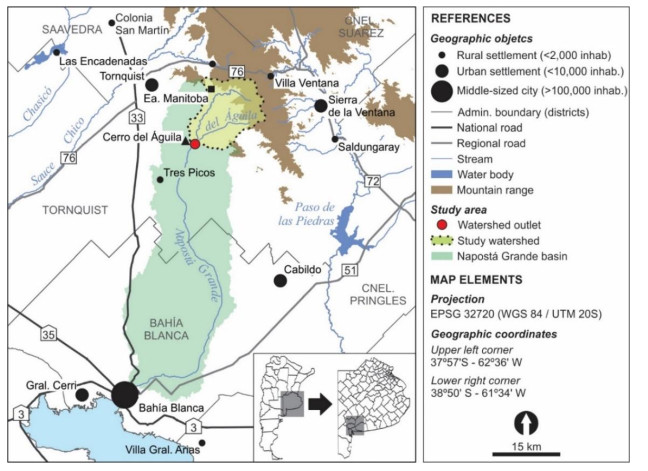
This paper examined and compared the reliability of two popular unit hydrograph methods for flood assessment in a dryland, poorly gauged basin: the Soil Conservation Service (NRCS-UH) method and the geomorphologic instantaneous unit hydrograph (GIUH) model. In addition, two different estimates of the basin's time of concentration were compared, along with varying values of the runoff curve number, to compute the watershed lag. Simulations were performed for the upper Napostá Grande (SW Buenos Aires, Argentina), using eight historic rainfall-runoff events to validate the resulting hydrograph at the basin outlet. Validation used runoff volume, peak flow, and recession time as an alternative to time to peak, for which only mean daily data were available. Results revealed great discrepancies in unit hydrograph parameters for varying determination methods, time of concentration estimates, and basin lag factors, as well as lower-than-standard peak rate factors for GIUH hydrographs. The comparison of simulated with observed hydrographs suggested a better agreement of GIUH for the highest retardance factor, as it produced the smaller peaks with the longer recession. This study informs on the complex relationships involved in unit hydrograph (UH) determination for the studied basin and warns about the variability of obtained results depending on the applied methodology, the caution needed in the systematic use of standard parameters, and the importance of verifying the accuracy of results. This provides a valuable framework for flood assessment within regional, ungauged basins with similar characteristics, which may exhibit comparable total runoff volumes for the same rainfall event but not necessarily equivalent flood hydrographs.

References

[1]	Singh P, Mishra SK, Jain MK (2014) A review of the synthetic unit hydrograph: from the empirical UH to advanced geomorphological methods. Hydrol Sci J 59: 239–261. https://doi.org/10.1080/02626667.2013.870664 doi: 10.1080/02626667.2013.870664
[2]	Lasco JDD, Olivera F, Sharif HO (2022) Unit hydrograph peak rate factor estimation for Texas watersheds. J Hydrol Eng 27: 04022026. https://doi.org/10.1061/(ASCE)HE.1943-5584.0002212 doi: 10.1061/(ASCE)HE.1943-5584.0002212
[3]	Guo J (2022) General and analytic unit hydrograph and its applications. J Hydrol Eng 27: 04021046. https://doi.org/10.1061/(ASCE)HE.1943-5584.0002149 doi: 10.1061/(ASCE)HE.1943-5584.0002149
[4]	Zakizadeh F, Malekinezhad H (2015) Comparison of methods for estimation of flood hydrograph characteristics. Russ Meteorol Hydrol 40: 828–837. https://doi.org/10.3103/S1068373915120080 doi: 10.3103/S1068373915120080
[5]	Boonstra J (1994) Estimating peak runoff rates. In: Ritzema HP, editor. Drainage principles and applications. Wageningen: International Institute for Land Reclamation and Improvement. 111–144.
[6]	Natural Resources Conservation Service, Part 630: Hydrology, Chapter 16: Hydrographs. USDA. National Engineering Handbook National Engineering Handbook, 2007. Available from: https://policy.nrcs.usda.gov/searchdirective/PART%20630.
[7]	Barrios MI, Olaya EJ (2007) Calculo y análisis de hidrogramas para el flujo torrencial del 22 de Junio de 2006 ocurrido en la microcuenca "El Salto", Ibagué-Colombia. Avances en Recursos Hidráulicos, 31–40.
[8]	Jena S, Tiwari K (2006) Modeling synthetic unit hydrograph parameters with geomorphologic parameters of watersheds. J Hydrol 319: 1–14. https://doi.org/10.1016/j.jhydrol.2005.03.025 doi: 10.1016/j.jhydrol.2005.03.025
[9]	Kusumastuti DI, Jokowinarno D (2012) Time step issue in unit hydrograph for improving runoff prediction in small catchments. J Water Resour Prot 4: 686–693.
[10]	Pérez Cruz LM, Rubio Calderón LC (2019) Determinación del hidrograma unitario para la cuenca de la quebrada Padre De Jesús, Bogotá DC. Bogotá, Colombia: Universidad Distrital Francisco José de Caldas.
[11]	Callow J, Boggs G (2013) Studying reach-scale spatial hydrology in ungauged catchments. J Hydrol 496: 31–46. https://doi.org/10.1016/j.jhydrol.2013.05.030 doi: 10.1016/j.jhydrol.2013.05.030
[12]	McMahon TA, Vogel RM, Peel MC, et al. (2007) Global streamflows. Part 1: Characteristics of annual streamflows. J Hydrol 347: 243–259. https://doi.org/10.1016/j.jhydrol.2007.09.002 doi: 10.1016/j.jhydrol.2007.09.002
[13]	Coron L, Andréassian V, Perrin C, et al. (2012) Crash testing hydrological models in contrasted climate conditions: an experiment on 216 Australian catchments. Water Resour Res 48: W05552. https://doi.org/10.1029/2011WR011721
[14]	Huang T, Merwade V (2023) Developing Customized NRCS Unit Hydrographs (Finley UHs) for Ungauged Watersheds in Indiana. West Lafayette, In: Purdue University. https://doi.org/10.5703/1288284317644
[15]	Rodríguez Iturbe I, Valdés JB (1979) The geomorphologic structure of hydrologic response. Water Resour Res 15: 1409–1420. https://doi.org/10.1029/WR015i006p01409 doi: 10.1029/WR015i006p01409
[16]	Andrieu H, Moussa R, Kirstetter PE (2021) The Event-specific Geomorphological Instantaneous Unit Hydrograph (E-GIUH): The basin hydrological response characteristic of a flood event. J Hydrol 603: 127158. https://doi.org/10.1016/j.jhydrol.2021.127158 doi: 10.1016/j.jhydrol.2021.127158
[17]	Chen Y, Shi P, Ji X, et al. (2019) New method to calculate the dynamic factor-flow velocity in Geomorphologic instantaneous unit hydrograph. Sci Rep 9: 14201. https://doi.org/10.1038/s41598-019-50723-x doi: 10.1038/s41598-019-50723-x
[18]	Iguacel NA, Aguinaga Martínez M, López NC, et al. (2022) Metodología recomendada para la obtención de hidrogramas unitarios de un arroyo del SO bonaerense instrumentado. Memorias del Encuentro Argentino de Ingeniería (6℃ADI–12℃AEDI). Corrientes, Argentina: Universidad de la Cuenca del Plata, 1663–1669. Available from: https://confedi.org.ar/download/Libro-de-Actas-6toCADI-12CAEDI.pdf.
[19]	López N, Casado AL, Revollo Sarmiento NV, et al. (2023) Potencial de escorrentía en función del número de curva en una cuenca serrana, Napostá Grande (Argentina). Geociências 42: 402–418. https://doi.org/10.5016/geociencias.v42i3.17188 doi: 10.5016/geociencias.v42i3.17188
[20]	Instituto Nacional de Estadística y Censos, Encuesta Permanente de Hogares. Cuadros regulares—EPH Continua. In: Censo INdEy. 2020. Available from: https://www.indec.gob.ar/indec/web/Institucional-Indec-bases_EPH_tabulado_continua.
[21]	Instituto Nacional de Estadística y Censos (2022) Censo nacional de población, hogares y viviendas 2022: resultados provisionales. In: Censo INdEy.
[22]	Casado A, Campo AM (2019) Extremos hidroclimáticos y recursos hídricos: estado de conocimiento en el suroeste bonaerense, Argentina. Cuadernos Geográficos 58: 6–26.
[23]	Berón de la Puente F, Gil V, Zapperi P (2017) Estimación de la pérdida del suelo por erosión hídrica de la cuenca alta del arroyo Napostá Grande, Buenos Aires, Argentina. Departamento de Geografía y Turismo, Universidad Nacional del Sur—CONICET.
[24]	Scian B (2000) Episodios ENSO y su relación con las anomalías de precipitación en la pradera pampeana. Geoacta 25: 23–40.
[25]	Scian B, Labraga JC, Reimers W, et al. (2006) Characteristics of large-scale atmospheric circulation related to extreme monthly rainfall anomalies in the Pampa Region, Argentina, under non-ENSO conditions. Theor Appl Climatol 85: 89–106. https://doi.org/10.1007/s00704-005-0182-8 doi: 10.1007/s00704-005-0182-8
[26]	Carrica JC, Lexow C (2004) Evaluación de la recarga natural al acuífero de la cuenca superior del arroyo Napostá Grande, provincia de Buenos Aires. Rev Asoc Geol Argent 59: 281–290.
[27]	Carrica J (1998) Hidrogeología de la cuenca del arroyo Napostá Grande. Provincia de Buenos Aires (Tesis doctoral inédita), Universidad Nacional del Sur, Departamento de Geología, Bahía Blanca.
[28]	Sloto RA, Crouse MY (1996) HYSEP, a computer program for streamflow hydrograph separation and analysis. U.S. Geological Survey Water-Resources Investigations Report 1996–4040, 46. https://doi.org/10.3133/wri964040
[29]	Curtis JA, Burns ER, Sando R (2020) Regional patterns in hydrologic response, a new three-component metric for hydrograph analysis and implications for ecohydrology, Northwest Volcanic Aquifer Study Area, USA. J Hydrol Reg Stud 30: 100698. https://doi.org/10.1016/j.ejrh.2020.100698 doi: 10.1016/j.ejrh.2020.100698
[30]	Carrica J, Bonorino G (2000) Estimación de la recarga mediante el análisis de las curvas de recesión de hidrogramas fluviales. Águas Subterrâneas 2000: 23494.
[31]	Carrica J, Robledo C (2002) Cálculo de la recarga de acuíferos mediante el análisis de las curvas de recesión de hidrogramas fluviales compuestos. Geoacta 27: 16–29. http://sedici.unlp.edu.ar/handle/10915/140480
[32]	Hawkins RH, Hjelmfelt Jr AT, Zevenbergen AW (1985) Runoff probability, storm depth, and curve numbers. J Irrig Drain Eng 111: 330–340. https://doi.org/10.1061/(ASCE)0733-9437(1985)111:4(330) doi: 10.1061/(ASCE)0733-9437(1985)111:4(330)
[33]	Strahler AN (1957) Quantitative analysis of watershed geomorphology. Eos Trans Am Geophys Union 38: 913–920. https://doi.org/10.1029/TR038i006p00913 doi: 10.1029/TR038i006p00913
[34]	USACE, Hydrologic Modeling System HEC-HMS User's Manual. Davis, CA, USA: Hydrologic Engineering Center, U.S. Army Corps of Engineers, 2023. 658. Available from: https://www.hec.usace.army.mil/confluence/hmsdocs/hmsum/4.11.
[35]	Zavoianu I (1985) Morphometry of drainage basins, Serie 20: developments in water science. Amsterdam/Bucharest: Elsevier/Editura Academiei.
[36]	Schumm SA (1956) Evolution of drainage systems and slopes in badlands at Perth Amboy, New Jersey. Geol Soc Am Bull 67: 597–646. https://doi.org/10.1130/0016-7606(1956)67[597:EODSAS]2.0.CO; 2 doi: 10.1130/0016-7606(1956)67[597:EODSAS]2.0.CO;2
[37]	Horton RE (1945) Erosional development of streams and their drainage basins: hydrophysical approach to quantitative morphology. Bull Geol Soc Am 56: 275–370. https://doi.org/10.1130/0016-7606(1945)56[275:EDOSAT]2.0.CO; 2 doi: 10.1130/0016-7606(1945)56[275:EDOSAT]2.0.CO;2
[38]	Natural Resources Conservation Service, Part 630: Hydrology, Chapter 15: Time of concentration. Washington DC, USA: Natural Resources Conservation Service, USDA, 2010. 29. Available from: https://policy.nrcs.usda.gov/searchdirective/PART%20630.
[39]	Kirpich ZP (1940) Time of concentration of small agricultural watersheds. Civ Eng 10: 362.
[40]	Hawkins RH (2014) Curve number method: Time to think anew? J Hydrol Eng 19: 1059–1059. https://doi.org/10.1061/(ASCE)HE.1943-5584.0000954 doi: 10.1061/(ASCE)HE.1943-5584.0000954
[41]	Hawkins RH, Ward TJ, Woodward DE, et al. (2009) Curve number hydrology: State of the practice: American Society of Civil Engineers.
[42]	Rodríguez-Iturbe I, Devoto G, Valdés JB (1979) Discharge response analysis and hydrologic similarity: the interrelation between the geomorphologic IUH and the storm characteristics. Water Resour Res 15: 1435–1444. https://doi.org/10.1029/WR015i006p01435 doi: 10.1029/WR015i006p01435
[43]	Pedroso A, Mannich M (2021) The uncertainties of synthetic unit hydrographs applied for basins with different runoff generation processes. RBRH 26: e38. https://doi.org/10.1590/2318-0331.262120210093
[44]	Wilkening H (1990) Procedure for selection of SCS peak rate factors for use in MSSW permit applications. Florida, US: St. Johns River Water Management District. Memorandum SJRWMD Memorandum SJRWMD. Available from: https://www.devoeng.com/memos/unit_hydrograph_shape_factor_memo_from_SJRWMD.pdf.
[45]	Oudin L, Andréassian V, Perrin C, et al. (2008) Spatial proximity, physical similarity, regression and ungaged catchments: A comparison of regionalization approaches based on 913 French catchments. Water Resour Res 44. https://doi.org/10.1029/2007WR006240
[46]	Tegegne G, Kim YO (2018) Modelling ungauged catchments using the catchment runoff response similarity. J Hydrol 564: 452–466. https://doi.org/10.1016/j.jhydrol.2018.07.042 doi: 10.1016/j.jhydrol.2018.07.042

Reader Comments

Your name:*

Email:*
© 2025 the Author(s), licensee AIMS Press. This is an open access article distributed under the terms of the Creative Commons Attribution License (http://creativecommons.org/licenses/by/4.0)