In the realm of Unsupervised Domain Adaptation (UDA), adversarial learning has achieved significant progress. Existing adversarial UDA methods typically employ additional discriminators and feature extractors to engage in a max-min game. However, these methods often fail to effectively utilize the predicted discriminative information, thus resulting in the mode collapse of the generator. In this paper, we propose a Dynamic Balance-based Domain Adaptation (DBDA) method for self-correlated domain adaptive image classification. Instead of adding extra discriminators, we repurpose the classifier as a discriminator and introduce a dynamic balancing learning approach. This approach ensures an explicit domain alignment and category distinction, thus enabling DBDA to fully leverage the predicted discriminative information for an effective feature alignment. We conducted experiments on multiple datasets, therefore demonstrating that the proposed method maintains a robust classification performance across various scenarios.
Citation: Hui Jiang, Di Wu, Xing Wei, Wenhao Jiang, Xiongbo Qing. Discriminator-free adversarial domain adaptation with information balance[J]. Electronic Research Archive, 2025, 33(1): 210-230. doi: 10.3934/era.2025011
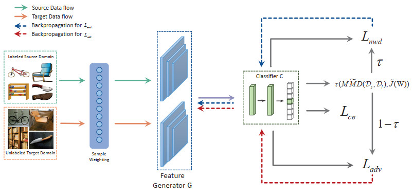
In the realm of Unsupervised Domain Adaptation (UDA), adversarial learning has achieved significant progress. Existing adversarial UDA methods typically employ additional discriminators and feature extractors to engage in a max-min game. However, these methods often fail to effectively utilize the predicted discriminative information, thus resulting in the mode collapse of the generator. In this paper, we propose a Dynamic Balance-based Domain Adaptation (DBDA) method for self-correlated domain adaptive image classification. Instead of adding extra discriminators, we repurpose the classifier as a discriminator and introduce a dynamic balancing learning approach. This approach ensures an explicit domain alignment and category distinction, thus enabling DBDA to fully leverage the predicted discriminative information for an effective feature alignment. We conducted experiments on multiple datasets, therefore demonstrating that the proposed method maintains a robust classification performance across various scenarios.

| [1] | L. Zhu, L. L. Chan, T. K. Ng, M. Zhang, B. C. Ooi, Deep co-training for cross-modality medical image segmentation, in ECAI 2023, 372 (2023), 3140–3147. https://doi.org/10.3233/FAIA230633 |
| [2] | Y. Ganin, V. Lempitsky, Unsupervised domain adaptation by backpropagation, in Proceedings of the 32nd International Conference on International Conference on Machine Learning, 37 (2015), 1180–1189. Available from: https://dl.acm.org/doi/10.5555/3045118.3045244. |
| [3] |
L. Abdi, S. Hashemi, Unsupervised domain adaptation based on correlation maximization, IEEE Access, 9 (2021), 127054–127067. https://doi.org/10.1109/ACCESS.2021.3111586 doi: 10.1109/ACCESS.2021.3111586

|
| [4] | H. Venkateswara, J. Eusebio, S. Chakraborty, S. Panchanathan, Deep hashing network for unsupervised domain adaptation, in 2017 IEEE/CVF Conference on Computer Vision and Pattern Recognition (CVPR), (2017), 5018–5027. https://doi.org/10.1109/CVPR.2017.572 |
| [5] | K. Saito, K. Watanabe, Y. Ushiku, T. Harada, Maximum classifier discrepancy for unsupervised domain adaptation, in 2018 IEEE/CVF Conference on Computer Vision and Pattern Recognition (CVPR), (2018), 3723–3732. https://doi.org/10.1109/CVPR.2018.00392 |
| [6] | B. Xie, L. Yuan, S. Li, C. H. Liu, X. Cheng, G. Wang, Active learning for domain adaptation: An energy-based approach, in Proceedings of the AAAI Conference on Artificial Intelligence, 36 (2022), 8708–8716. https://doi.org/10.1609/aaai.v36i8.20850 |
| [7] | E. Tzeng, J. Hoffman, N. Zhang, K. Saenko, T. Darrell, Deep domain confusion: Maximizing for domain invariance, preprint, arXiv: 1412.3474. |
| [8] |
S. Li, S. Song, G. Huang, Z. Ding, C. Wu, Domain invariant and class discriminative feature learning for visual domain adaptation, IEEE Trans. Image Process., 27 (2018), 4260–4273. https://doi.org/10.1109/TIP.2018.2839528 doi: 10.1109/TIP.2018.2839528
|
| [9] | Z. Du, J. Li, H. Su, L. Zhu, K. Lu, Cross-domain gradient discrepancy minimization for unsupervised domain adaptation, in 2021 IEEE/CVF Conference on Computer Vision and Pattern Recognition (CVPR), (2021), 3937–3946. https://doi.org/10.1109/CVPR46437.2021.00393 |
| [10] | T. Chen, S. Kornblith, M. Norouzi, G. Hinton, A simple framework for contrastive learning of visual representations, in Proceedings of the 37th International Conference on Machine Learning, 119 (2020), 1597–1607. |
| [11] | C. Park, J. Lee, J. Yoo, M. Hur, S. Yoon, Joint contrastive learning for unsupervised domain adaptation, preprint, arXiv: 2006.10297. |
| [12] |
Y. Ganin, E. Ustinova, H. Ajakan, P. Germain, H. Larochelle, F. Laviolette, et al., Domain-adversarial training of neural networks, J. Mach. Learn. Res., 17 (2016), 1–35. https://doi.org/10.1007/978-3-319-58347-1_10 doi: 10.1007/978-3-319-58347-1_10
|
| [13] | H. Tang, K. Jia, Discriminative adversarial domain adaptation, in Proceedings of the AAAI Conference on Artificial Intelligence, 34 (2020), 5940–5947. https://doi.org/10.1609/aaai.v34i04.6054 |
| [14] | N. Carion, F. Massa, G. Synnaeve, N. Usunier, A. Kirillov, S. Zagoruyko, End-to-end object detection with transformers, in European Conference on Computer Vision, 12346 (2020), 213–229. https://doi.org/10.1007/978-3-030-58452-8_13 |
| [15] | Z. Gao, S. Zhang, K. Huang, Q. Wang, C. Zhong, Gradient distribution alignment certificates better adversarial domain adaptation, in 2021 IEEE/CVF International Conference on Computer Vision, (2021), 8937–8946. https://doi.org/10.1109/ICCV48922.2021.00881 |
| [16] | H. Liu, M. Long, J. Wang, M. Jordan, Transferable adversarial training: A general approach to adapting deep classifiers, in Proceedings of the 36th International Conference on Machine Learning, 97 (2019), 4013–4022. Available from: https://proceedings.mlr.press/v97/liu19b.html. |
| [17] | M. Xu, J. Zhang, B. Ni, T. Li, C. Wang, Q. Tian, et al., Adversarial domain adaptation with domain mixup, in Proceedings of the AAAI Conference on Artificial Intelligence, 34 (2020), 6502–6509. https://doi.org/10.1609/aaai.v34i04.6123 |
| [18] | M. Long, Z. Cao, J. Wang, M. I. Jordan, Conditional adversarial domain adaptation, in Proceedings of the 32nd International Conference on Neural Information Processing Systems, 31 (2018), 1647–1657. Available from: https://dl.acm.org/doi/10.5555/3326943.3327094. |
| [19] | M. Mirza, S. Osindero, Conditional generative adversarial nets, preprint, arXiv: 1411.1784. |
| [20] | X. Chen, S. Wang, M. Long, J. Wang, Transferability vs. discriminability: Batch spectral penalization for adversarial domain adaptation, in Proceedings of the 36th International Conference on Machine Learning, 97 (2019), 1081–1090. Available from: https://proceedings.mlr.press/v97/chen19i.html. |
| [21] | M. Long, Y. Cao, J. Wang, M. Jordan, Learning transferable features with deep adaptation networks, in Proceedings of the 32nd International Conference on Machine Learning, 37 (2015), 97–105. |
| [22] |
C. X. Ren, Y. W. Luo, D. Q. Dai, BuresNet: Conditional bures metric for transferable representation learning, IEEE Trans. Pattern Anal. Mach. Intell., 45 (2022), 4198–4213. https://doi.org/10.1109/TPAMI.2022.3190645 doi: 10.1109/TPAMI.2022.3190645
|
| [23] | K. Shen, R. M. Jones, A. Kumar, S. M. Xie, J. Z. Haochen, T. Ma, et al., Connect, not collapse: Explaining contrastive learning for unsupervised domain adaptation, in Proceedings of the 39th International Conference on Machine Learning, 162 (2022), 19847–19878. |
| [24] | M. Thota, G. Leontidis, Contrastive domain adaptation, in 2021 IEEE/CVF Conference on Computer Vision and Pattern Recognition Workshops (CVPRW), (2021), 2209–2218. https://doi.org/10.1109/CVPRW53098.2021.00250 |
| [25] | Y. Wang, Y. Li, S. Li, W. Song, J. Fan, S. Gao, et al., Deep graph mutual learning for cross-domain recommendation, in International Conference on Database Systems for Advanced Applications, 13246 (2022), 298–305. https://doi.org/10.1007/978-3-031-00126-0_22 |
| [26] | Y. Wang, Y. Song, S. Li, C. Cheng, W. Ju, M. Zhang, et al., Disencite: Graph-based disentangled representation learning for context-specific citation generation, in Proceedings of the AAAI Conference on Artificial Intelligence, 36 (2022), 11449–11458. https://doi.org/10.1609/aaai.v36i10.21397 |
| [27] | Y. Wang, X. Luo, C. Chen, X. S. Hua, M. Zhang, W. Ju, DisenSemi: Semi-supervised graph classification via disentangled representation learning, IEEE Trans. Neural Networks Learn. Syst., (2024), 1–13. https://doi.org/10.1109/tnnls.2024.3431871 |
| [28] | Y. Wang, Y. Qin, F. Sun, B. Zhang, X. Hou, K. Hu, et al., DisenCTR: Dynamic graph-based disentangled representation for click-through rate prediction, in Proceedings of the 45th International ACM SIGIR Conference on Research and Development in Information Retrieval, (2022), 2314–2318. https://doi.org/10.1145/3477495.3531851 |
| [29] | Y. Wang, S. Tang, Y. Lei, W. Song, S. Wang, M. Zhang, Disenhan: Disentangled heterogeneous graph attention network for recommendation, in Proceedings of the 29th ACM International Conference on Information & Knowledge Management, (2020), 1605–1614. https://doi.org/10.1145/3340531.3411996 |
| [30] | I. Goodfellow, J. Pouget-Abadie, M. Mirza, B. Xu, D. Warde-Farley, S. Ozair, et al., Generative adversarial nets, in Proceedings of the 27th International Conference on Neural Information Processing Systems, 27 (2014). Available from: https://dl.acm.org/doi/10.5555/2969033.2969125. |
| [31] | M. Long, H. Zhu, J. Wang, M. I. Jordan, Deep transfer learning with joint adaptation networks, in Proceedings of the 34th International Conference on Machine Learning, 70 (2017), 2208–2217. |
| [32] |
C. Zhu, Q. Wang, Y. Xie, S. Xu, Multiview latent space learning with progressively fine-tuned deep features for unsupervised domain adaptation, Inf. Sci., 662 (2024), 120223. https://doi.org/10.1016/j.ins.2024.120223 doi: 10.1016/j.ins.2024.120223
|
| [33] | X. Liu, S. Zhang, Graph consistency based mean-teaching for unsupervised domain adaptive person re-identification, preprint, arXiv: 2105.04776. |
| [34] |
C. Zhu, L. Zhang, W. Luo, G. Jiang, Q. Wang, Tensorial multiview low-rank high-order graph learning for context-enhanced domain adaptation, Neural Networks, 181 (2024), 106859. https://doi.org/10.1016/j.neunet.2024.106859 doi: 10.1016/j.neunet.2024.106859
|
| [35] | I. P. Singh, E. Ghorbel, A. Kacem, A. Rathinam, D. Aouada, Discriminator-free unsupervised domain adaptation for multi-label image classification, in 2024 IEEE/CVF Winter Conference on Applications of Computer Vision (WACV), (2024), 3924–3933. https://doi.org/10.1109/wacv57701.2024.00389 |
| [36] | Z. Chen, J. Wei, R. Li, Unsupervised multi-modal medical image registration via discriminator-free image-to-image translation, in Proceedings of the Thirty-First International Joint Conference on Artificial Intelligence, (2022), 834–840. https://doi.org/10.24963/ijcai.2022/117 |
| [37] |
J. Wang, Y. Chen, W. Feng, H. Yu, M. Huang, Q. Yang, Transfer learning with dynamic distribution adaptation, ACM Trans. Intell. Syst. Technol., 11 (2020), 2157–6904. https://doi.org/10.1145/3360309 doi: 10.1145/3360309
|
| [38] | Y. Li, L. Yuan, Y. Chen, P. Wang, N. Vasconcelos, Dynamic transfer for multi-source domain adaptation, in 2021 IEEE/CVF Conference on Computer Vision and Pattern Recognition (CVPR), (2021), 10993–11002. https://doi.org/10.1109/cvpr46437.2021.01085 |
| [39] | K. Saenko, B. Kulis, M. Fritz, T. Darrell, Adapting visual category models to new domains, in Computer Vision–ECCV 2010: 11th European Conference on Computer Vision, 6314 (2010), 213–226. https://doi.org/10.1007/978-3-642-15561-1_16 |
| [40] | X. Peng, B. Usman, N. Kaushik, J. Hoffman, D. Wang, K. Saenko, Visda: The visual domain adaptation challenge, preprint, arXiv: 1710.06924. |
| [41] | K. He, X. Zhang, S. Ren, J. Sun, Deep residual learning for image recognition, in 2016 IEEE Conference on Computer Vision and Pattern Recognition (CVPR), (2016), 770–778. https://doi.org/10.1109/CVPR.2016.90 |
| [42] | J. Shen, Y. Qu, W. Zhang, Y. Yu, Wasserstein distance guided representation learning for domain adaptation, in Proceedings of the AAAI Conference on Artificial Intelligence, 32 (2018). https://doi.org/10.1609/aaai.v32i1.11784 |
| [43] | R. Xu, G. Li, J. Yang, L. Lin, Larger norm more transferable: An adaptive feature norm approach for unsupervised domain adaptation, in 2019 IEEE/CVF International Conference on Computer Vision, (2019), 1426–1435. https://doi.org/10.1109/ICCV.2019.00151 |
| [44] | M. Li, Y. M. Zhai, Y. W. Luo, P. F. Ge, C. X. Ren, Enhanced transport distance for unsupervised domain adaptation, in 2020 IEEE/CVF Conference on Computer Vision and Pattern Recognition (CVPR), (2020), 13936–13944. https://doi.org/10.1109/CVPR42600.2020.01395 |
| [45] |
J. Li, Z. Li, S. Lü, Feature concatenation for adversarial domain adaptation, Expert Syst. Appl., 169 (2021), 114490. https://doi.org/10.1016/j.eswa.2020.114490 doi: 10.1016/j.eswa.2020.114490
|
| [46] |
Y. Li, Y. Liu, D. Zheng, Y. Huang, Y. Tang, Discriminable feature enhancement for unsupervised domain adaptation, Image Vision Comput., 137 (2023), 104755. https://doi.org/10.1016/j.imavis.2023.104755 doi: 10.1016/j.imavis.2023.104755
|
| [47] |
S. Yao, Q. Kang, M. Zhou, M. J. Rawa, A. Albeshri, Discriminative manifold distribution alignment for domain adaptation, IEEE Trans. Syst. Man Cybern.: Syst., 53 (2022), 1183–1197. https://doi.org/10.1109/TSMC.2022.3195239 doi: 10.1109/TSMC.2022.3195239
|
| [48] |
Q. Tian, H. Yang, Z. Lu, M. Liu, Unsupervised domain adaptation through adversarial enhancement and gradient discrepancy minimization, Comput. Electr. Eng., 105 (2023), 108483. https://doi.org/10.1016/j.compeleceng.2022.108483 doi: 10.1016/j.compeleceng.2022.108483
|
| [49] | Z. Deng, Y. Luo, J. Zhu, Cluster alignment with a teacher for unsupervised domain adaptation, in 2019 IEEE/CVF International Conference on Computer Vision, (2019), 9944–9953. https://doi.org/10.1109/ICCV.2019.01004 |
| [50] |
P. Liu, T. Xiao, C. Fan, W. Zhao, X. Tang, H. Liu, Importance-weighted conditional adversarial network for unsupervised domain adaptation, Expert Syst. Appl., 155 (2020), 113404. https://doi.org/10.1016/j.eswa.2020.113404 doi: 10.1016/j.eswa.2020.113404
|
| [51] |
X. Wu, S. Zhang, Q. Zhou, Z. Yang, C. Zhao, L. J. Latecki, Entropy minimization versus diversity maximization for domain adaptation, IEEE Trans. Neural Networks Learn. Syst., 34 (2021), 2896–2907. https://doi.org/10.1109/TNNLS.2021.3110109 doi: 10.1109/TNNLS.2021.3110109
|
| [52] | E. Tzeng, J. Hoffman, K. Saenko, T. Darrell, Adversarial discriminative domain adaptation, in 2017 IEEE Conference on Computer Vision and Pattern Recognition (CVPR), (2017), 7167–7176. https://doi.org/10.1109/cvpr.2017.316 |
| [53] | Z. Pei, Z. Cao, M. Long, J. Wang, Multi-adversarial domain adaptation, in Proceedings of the AAAI Conference on Artificial Intelligence, 32 (2018). https://doi.org/10.1609/aaai.v32i1.11767 |
| [54] |
Q. Tian, J. Zhou, Y. Chu, Joint bi-adversarial learning for unsupervised domain adaptation, Knowledge-Based Syst., 248 (2022), 108903. https://doi.org/10.1016/j.knosys.2022.108903 doi: 10.1016/j.knosys.2022.108903
|
| [55] |
J. Gu, X. Qian, Q. Zhang, H. Zhang, F. Wu, Unsupervised domain adaptation for covid-19 classification based on balanced slice wasserstein distance, Comput. Biol. Med., 164 (2023), 107207. https://doi.org/10.1016/j.compbiomed.2023.107207 doi: 10.1016/j.compbiomed.2023.107207
|
| [56] | Z. Yue, Q. Sun, X. S. Hua, H. Zhang, Transporting causal mechanisms for unsupervised domain adaptation, in 2021 IEEE/CVF International Conference on Computer Vision (ICCV), (2021), 8599–8608. https://doi.org/10.1109/ICCV48922.2021.00848 |


Figures(4) / Tables(6)
Hui Jiang, Di Wu, Xing Wei, Wenhao Jiang, Xiongbo Qing. Discriminator-free adversarial domain adaptation with information balance[J]. Electronic Research Archive, 2025, 33(1): 210-230. doi: 10.3934/era.2025011


 DownLoad: