A hybrid singular value thresholding algorithm with diagonal-modify for low-rank matrix recovery

Ruiping Wen; Liang Zhang; Yalei Pei; Ruiping Wen; Liang Zhang; Yalei Pei

doi:10.3934/era.2024274

Electronic Research Archive

2024, Volume 32, Issue 11: 5926-5942. doi: 10.3934/era.2024274

Previous Article Next Article

Research article

A hybrid singular value thresholding algorithm with diagonal-modify for low-rank matrix recovery

1.
Shanxi Key Laboratory for Intelligent Optimization Computing and Block-chain Technology, Taiyuan Normal University, Jinzhong 030619, China
2.
School of Mathematics and Statistics, Taiyuan Normal University, Jinzhong 030619, China

Received: 21 September 2024 Revised: 21 October 2024 Accepted: 24 October 2024 Published: 04 November 2024

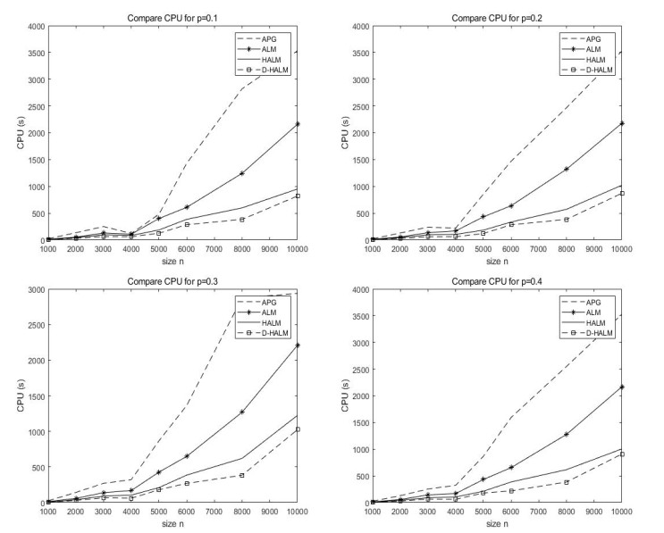
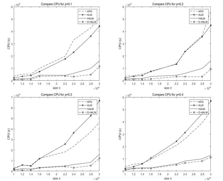
In this paper, a new hybrid singular value thresholding with diagonal-modify algorithm based on the augmented Lagrange multiplier (ALM) method was proposed for low-rank matrix recovery, in which only part singular values were treated by a hybrid threshold operator with diagonal-update, and which allowed the algorithm to make use of simple arithmetic operation and keep the computational cost of each iteration low. The new algorithm decreased the complexity of the singular value decomposition and shortened the computing time. The convergence of the new algorithm was discussed. Finally, numerical experiments shown that the new algorithm greatly improved the solving efficiency of a matrix recovery problem and saved the calculation cost, and its effect was obviously better than that of the other algorithms mentioned in experiments.
- low-rank matrix recovery,
- augmented Lagrange multiplier,
- diagonal-modify,
- hybrid singular value threshold
Citation: Ruiping Wen, Liang Zhang, Yalei Pei. A hybrid singular value thresholding algorithm with diagonal-modify for low-rank matrix recovery[J]. Electronic Research Archive, 2024, 32(11): 5926-5942. doi: 10.3934/era.2024274

Related Papers:

Abstract

In this paper, a new hybrid singular value thresholding with diagonal-modify algorithm based on the augmented Lagrange multiplier (ALM) method was proposed for low-rank matrix recovery, in which only part singular values were treated by a hybrid threshold operator with diagonal-update, and which allowed the algorithm to make use of simple arithmetic operation and keep the computational cost of each iteration low. The new algorithm decreased the complexity of the singular value decomposition and shortened the computing time. The convergence of the new algorithm was discussed. Finally, numerical experiments shown that the new algorithm greatly improved the solving efficiency of a matrix recovery problem and saved the calculation cost, and its effect was obviously better than that of the other algorithms mentioned in experiments.

References

[1]	A. Mongia, A. Majumdar, Matrix completion on multiple graphs: Application in collaborative filter- ing, Signal Process., 165 (2019), 144–148. https://doi.org/10.1016/j.sigpro.2019.07.002 doi: 10.1016/j.sigpro.2019.07.002
[2]	S. Daei, F. Haddadi, A. Amini, Exploitation prior information in block sprase signal, IEEE Trans. Signal Process., 99 (2018). https://doi.org/10.1109/TSP.2019.2931209 doi: 10.1109/TSP.2019.2931209
[3]	Z. Zhang, K. Zhao, H. Zha, Inducible regularization for low-rank matrix factorizations for collaborative filtering, Neurocomputing, 97 (2012), 52–62. https://doi.org/10.1016/j.neucom.2012.05.010 doi: 10.1016/j.neucom.2012.05.010
[4]	S. Li, Q. Li, Z. Zhu, G. Tang, M. B. Wakin, The global geometry of centralized and distributed low- rank matrix recovery without regularization, IEEE Signal Process. Lett., 27 (2020), 1400–1404. https://doi.org/10.1109/LSP.2020.3008876 doi: 10.1109/LSP.2020.3008876
[5]	B. J. Han, J. Y. Simg, Glass reflection removal using co-saliency based image alignment and low- rank matrix completion in gradient domain, IEEE Trans. Image Process., 27 (2018), 1–1. https://doi.org/10.1109/TIP.2018.2849880. doi: 10.1109/TIP.2018.2849880
[6]	L. I. Jie, F. Chen, Y. Wang, J. I. Fei, Y. U. Hua, Spatial spectrum estimation of incoherently dis tributed sources based on low-rank matrix recovery, IEEE Trans. Veh. Technol., 99 (2020). https://doi.org/10.1109/TVT.2020.2986783 doi: 10.1109/TVT.2020.2986783
[7]	Z. H. Zhu, Q. W. Tang, G. G. Wakin, B. Michael, Global optimality in low-rank matrix optimization, IEEE Trans. Signal Process., 66 (2018), 3614–3628. https://doi.org/10.1109/TSP.2018.2835403 doi: 10.1109/TSP.2018.2835403
[8]	M. Kech, M. Wolf, Constrained quantum tomography of semi-algebraic sets with applications to low-rank matrix recovery, Mathematics, 6 (2017), 171–195. https://doi.org/10.1093/imaiai/iaw019 doi: 10.1093/imaiai/iaw019
[9]	E. J. Candès, B. Recht, Exact low-rank matrix completion via convex optimization, in 2008 46th Annual Allerton Conference on Communication, Control, and Computing, (2009), 806–812. https://doi.org/10.1109/ALLERTON.2008.4797640
[10]	E. J. Candès, T. Tao, The power of convex relaxation: Near-optimal matrix completion, IEEE Trans. Inf. Theory, 56 (2010), 2053–2080. https://doi.org/10.1109/TIT.2010.2044061 doi: 10.1109/TIT.2010.2044061
[11]	B. Recht, A simpler approach to matrix completion, J. Mach. Learn. Res., 12 (2009), 3413–3430. https://doi.org/10.1177/0959651810397461 doi: 10.1177/0959651810397461
[12]	B. Recht, M. Fazel, P. A. Parrilo, Guaranteed minimum-rank solutions of linear matrix equations via nuclear norm minimization, SIAM Rev., 52 (2010), 471–501. https://doi.org/10.1137/070697835 doi: 10.1137/070697835
[13]	D. Gross, Recovering low-rank matrices from few coefficients in any basis, IEEE Trans Inf. Theory, 57 (2011), 1548–1566. https://doi.org/10.1109/TIT.2011.2104999 doi: 10.1109/TIT.2011.2104999
[14]	J. Wright, A. Ganesh, S. Rao, Y. Ma, Robust principal component analysis: exact recovery of corrupted low-rank matrices, in Neural Networks for Signal Processing X. Proceedings of the 2000 IEEE Signal Processing Society Workshop, 2009. https://doi.org/10.1109/NNSP.2000.889420
[15]	R. Meka, P. Jain, I. Dhillon, Guaranteed rank minimization via singular value projection, preprint, arXiv: 0909.5457. https://doi.org/10.48550/arXiv.0909.5457
[16]	A. Ganesh, Z. Lin, J. Wright, L. Wu, M. Chen, Y. Ma, Fast algorithms for recovering a corrupted low-rank matrix, in 2009 3rd IEEE International Workshop on Computational Advances in Multi-Sensor Adaptive Processing (CAMSAP), 2009. https://doi.org/10.1109/CAMSAP.2009.5413299.
[17]	J. F. Cai, E. J. Candès, Z. Shen, A singular value thresholding algorithm for matrix completion, SIAM J. Optim., 20 (2010), 1956–1982. https://doi.org/10.1137/080738970 doi: 10.1137/080738970
[18]	Z. Lin, A. Ganesh, J. Wright, L. Wu, M. Chen, Y. Ma, Fast convex optimization algorithms for exact recovery of a corrupted low-rank matrix, Coordinated Science Laboratory Report no. UILU-ENG-09-2214, DC-246, 2009. https://doi.org/10.1017/S0025315400020749
[19]	Z. Lin, M. Chen, Y. Ma, The augmented lagrange multiplier method for exact recovery of corrupted low-rank matrices, preprint, arXiv: 1009.5055. https://doi.org/10.48550/arXiv.1009.5055
[20]	J. Guo, R. P. Wen, Hybrid augmented lagrange multiplier algorithm for low-rank matrix com- pletion, Numer. Math.: Theory, Methods Appl., 44 (2022), 187–201.
[21]	G. H. Golub, C. F. Van Loan, Matrix Computations, 4^th edition, Johns Hopkins Studies in Mathematical Sciences, 2013.
[22]	D. Goldfarb, S. Ma, Convergence of fixed-point continuation algorithms for matrix rank minimization, Found. Comput. Math., 11 (2011), 183–210. https://doi.org/10.1007/s10208-011-9084-6 doi: 10.1007/s10208-011-9084-6

Reader Comments

Your name:*

Email:*
© 2024 the Author(s), licensee AIMS Press. This is an open access article distributed under the terms of the Creative Commons Attribution License (http://creativecommons.org/licenses/by/4.0)