


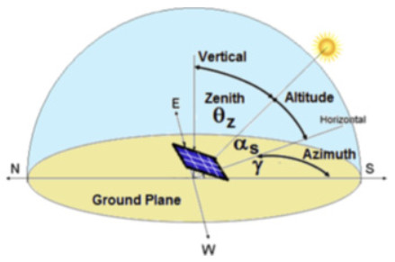
Figure 1.
Schematic representation of the solar azimuth angles [51].
The aim of this study was to build a regression model of solar irradiation in the Kulluk region of Turkey by using the multivariate adaptive regression splines (MARS) technique. Using the well-known data mining algorithm, MARS, this study has explored a convenient prediction model for continuous response variables, i.e., average daily energy production from the given system (Ed), average monthly energy production from given system (Em), average daily sum of global irradiation per square meter (Hd) and average annual sum of global irradiation per square meter (Hm). Four continuous estimators are included to estimate Ed, Em, Hd and Hm: Estimated losses due to temperature and low irradiance (ESLOTEM), estimated loss due to angular reflection effect (ESLOANGREF), combined photovoltaic system loss (COMPVLOSS) and rated power of the photovoltaic system (PPVS). Four prediction models as constructed by implementing the MARS algorithm, have been obtained by applying the smallest generalized cross-validation (GCV) criterion where the means of penalty are defined as 1 and the backward pruning method for the package "earth" of R software is used. As a result, it can be suggested that the procedure of the MARS algorithm, which achieves the greatest predictive accuracy of 100% or nearly 100%, permits researchers to obtain some remarkable hints for ascertaining predictors that affect solar irradiation parameters. The coefficient of determination denoted as R2 was estimated at the highest predictive accuracy to be nearly 1 for Ed, Em, Hd and Hm while the GCV values were found to be 0.000009, 0.018908, 0.000013 and 0.019021, respectively. The estimated results indicate that four MARS models with the first degree interaction effect have the best predictive performances for verification with the lowest GCV value.
Citation: Gokhan Sahin, W.G.J.H.M. Van Wilfried Sark. Estimation of most optimal azimuthal angles for maximum PV solar efficiency using multivariate adaptive regression splines (MARS)[J]. AIMS Energy, 2023, 11(6): 1328-1353. doi: 10.3934/energy.2023060
| [1] | Nadwan Majeed Ali, Handri Ammari . Design of a hybrid wind-solar street lighting system to power LED lights on highway poles. AIMS Energy, 2022, 10(2): 177-190. doi: 10.3934/energy.2022010 |
| [2] | Rami Al-Hajj, Ali Assi . Estimating solar irradiance using genetic programming technique and meteorological records. AIMS Energy, 2017, 5(5): 798-813. doi: 10.3934/energy.2017.5.798 |
| [3] | Sabir Rustemli, Zeki İlcihan, Gökhan Sahin, Wilfried G. J. H. M. van Sark . A novel design and simulation of a mechanical coordinate based photovoltaic solar tracking system. AIMS Energy, 2023, 11(5): 753-773. doi: 10.3934/energy.2023037 |
| [4] | Fadhil Khadoum Alhousni, Firas Basim Ismail, Paul C. Okonkwo, Hassan Mohamed, Bright O. Okonkwo, Omar A. Al-Shahri . A review of PV solar energy system operations and applications in Dhofar Oman. AIMS Energy, 2022, 10(4): 858-884. doi: 10.3934/energy.2022039 |
| [5] | Harry Ramenah, Philippe Casin, Moustapha Ba, Michel Benne, Camel Tanougast . Accurate determination of parameters relationship for photovoltaic power output by augmented dickey fuller test and engle granger method. AIMS Energy, 2018, 6(1): 19-48. doi: 10.3934/energy.2018.1.19 |
| [6] | Abdulrahman Th. Mohammad, Wisam A. M. Al-Shohani . Numerical and experimental investigation for analyzing the temperature influence on the performance of photovoltaic module. AIMS Energy, 2022, 10(5): 1026-1045. doi: 10.3934/energy.2022047 |
| [7] | Kaovinath Appalasamy, R Mamat, Sudhakar Kumarasamy . Smart thermal management of photovoltaic systems: Innovative strategies. AIMS Energy, 2025, 13(2): 309-353. doi: 10.3934/energy.2025013 |
| [8] | Michael O. Dioha, Atul Kumar . Rooftop solar PV for urban residential buildings of Nigeria: A preliminary attempt towards potential estimation. AIMS Energy, 2018, 6(5): 710-734. doi: 10.3934/energy.2018.5.710 |
| [9] | P. A. G. M. Amarasinghe, N. S. Abeygunawardana, T. N. Jayasekara, E. A. J. P. Edirisinghe, S. K. Abeygunawardane . Ensemble models for solar power forecasting—a weather classification approach. AIMS Energy, 2020, 8(2): 252-271. doi: 10.3934/energy.2020.2.252 |
| [10] | Muhammad Farhan Hanif, Muhammad Sabir Naveed, Mohamed Metwaly, Jicang Si, Xiangtao Liu, Jianchun Mi . Advancing solar energy forecasting with modified ANN and light GBM learning algorithms. AIMS Energy, 2024, 12(2): 350-386. doi: 10.3934/energy.2024017 |
The aim of this study was to build a regression model of solar irradiation in the Kulluk region of Turkey by using the multivariate adaptive regression splines (MARS) technique. Using the well-known data mining algorithm, MARS, this study has explored a convenient prediction model for continuous response variables, i.e., average daily energy production from the given system (Ed), average monthly energy production from given system (Em), average daily sum of global irradiation per square meter (Hd) and average annual sum of global irradiation per square meter (Hm). Four continuous estimators are included to estimate Ed, Em, Hd and Hm: Estimated losses due to temperature and low irradiance (ESLOTEM), estimated loss due to angular reflection effect (ESLOANGREF), combined photovoltaic system loss (COMPVLOSS) and rated power of the photovoltaic system (PPVS). Four prediction models as constructed by implementing the MARS algorithm, have been obtained by applying the smallest generalized cross-validation (GCV) criterion where the means of penalty are defined as 1 and the backward pruning method for the package "earth" of R software is used. As a result, it can be suggested that the procedure of the MARS algorithm, which achieves the greatest predictive accuracy of 100% or nearly 100%, permits researchers to obtain some remarkable hints for ascertaining predictors that affect solar irradiation parameters. The coefficient of determination denoted as R2 was estimated at the highest predictive accuracy to be nearly 1 for Ed, Em, Hd and Hm while the GCV values were found to be 0.000009, 0.018908, 0.000013 and 0.019021, respectively. The estimated results indicate that four MARS models with the first degree interaction effect have the best predictive performances for verification with the lowest GCV value.
According to the Global Status Report on Renewable Energy Sources [1], global renewable energy capacity reached 2,378 GW by the end of 2018, accounting for more than 33% of the world's total energy production. In 2018, new capacity additions were 55% from photovoltaic power systems, 28% from wind power systems and 11% from hydroelectric power. Photovoltaic power in particular reached a high level with nearly 100 GW added. Therefore, photovoltaic power generation became the world's fastest growing renewable energy source in 2022. In parallel with these developments, forecasting photovoltaic power generation has become an important requirement for energy trading. Different experimental methods have been used in the literature to model global solar irradiance, sunshine duration and air temperature data, which are important solar parameters in the installation of photovoltaic power systems. Despotovic et al. used a linear regression model to model monthly average daily diffuse solar irradiance, and the average absolute relative error was obtained as 0.060 [2]. Jamil and Akhtar used linear, logarithmic and exponential regression models for monthly average daily diffuse solar radiation modeling and the root mean square errors were found to be 0.8967, 1.1360 and 1.7705 MJ/m2, respectively [3]. Filho et al. calculated the root mean square error (RMSE) as 0.2718 MJ/m2 using a sigmoid logistic function in daily diffuse solar radiation modeling [4]. Liao et al. used a linear regression model to model the annual mean insolation duration and the coefficient of determination was 0.80 [5]. Chelbi et al. applied a linear regression model for monthly average daily insolation duration modeling and the coefficient of determination was found to be 0.7976 [6]. Zhu et al. applied a linear regression model for daily air temperature modeling and the RMSE was found to be 3.17 ℃ [7]. Ho et al. used a random forest regression model for daily maximum air temperature modeling and the mean absolute error was obtained as 1.67 ℃ [8]. Wenbin et al. used a sinusoidal curve fitting method for daily maximum and minimum air temperature modeling and calculated the correlation coefficients as 0.83 and 0.84, respectively [9]. Various machine learning, remote sensing and experimental models have been proposed in the literature to estimate solar radiation. Chang and Zhang improved the accuracy of hourly global solar irradiance estimation by using the hourly/daily irradiance ratio [10]. Jiang et al. extracted spatial patterns from satellite images by using convolutional neural networks, and they correlated them with hourly global solar irradiance using a multilayer perceptron. They realized accurate and reliable prediction [11]. Li et al. used a multivariate adaptive regression curve method to select the most important variables in meteorological data, and they realized good performance for the prediction of hourly global solar radiation on a horizontal surface [12]. Cornejo-Bueno et al. used different Gaussian processes, support vector regression and neural networks as machine learning regressors, and they demonstrated the effective performance of extreme learning machines in terms of hourly global solar radiation estimation [13]. Manju and Sandeep found surface measurement data to be more suitable than satellite measurement data for daily horizontal global solar radiation estimation [14]. Gouda et al. proposed a day-of-year-based hybrid sine and cosine wave model for the estimation of daily global solar radiation on a horizontal surface, and they obtained a good estimate without the need for any meteorological data [15]. Guermoui et al. proposed parallel and cascaded forecasting architectures based on weighted Gaussian process regression and improved the accuracy of daily global horizontal solar radiation forecasting [16]. Feng et al. compared temperature-based empirical and machine learning models in terms of their ability to predict daily horizontal global solar irradiance, and they recommended a hybrid mind evolution based artificial neural network model as the appropriate model [17]. With a theory of experimentation approach, Makade et al. identified altitude, relative humidity, and sunshine duration as the dominant parameters for monthly average horizontal global solar radiation estimation [18]. Kisi O. et al. demonstrated the efficiency of a dynamically evolving neural-fuzzy inference system in monthly average global solar radiation prediction [19]. Kaplan et al. developed cubic, quadratic and linear models based on the moving least squares approach and they obtained monthly average global solar radiation values that were in good agreement with real data [20]. Anis et al. designed generalized models based on sunshine duration to perform monthly average global solar radiation estimation and they identified the quartic function as the top ranked model in terms of global performance [21]. Gürel et al. used a feed-forward neural network, empirical models (three Angstrom-type models), the Holt-Winters time-series method and mathematical models to predict monthly average daily global solar radiation values. Pressure, relative humidity, wind speed, ambient temperature and sunshine duration data were used and the feedforward neural network was the most successful method with a coefficient of determination of 0.9911, RMSE of 0.78 and mean absolute percentage error (MAPE) of 4.9263% [22]. El-Baz et al. facilitated the integration of probabilistic forecasts into energy management system algorithms and demand side management algorithms. The forecasting ability improved to 48.6% relative to the continuum model [23]. Hu et al. used ground-based cloud imagery for ultra-short-term photovoltaic power forecasting. Using radial basis functions, mean absolute error (MAE) and MAPE values were reduced by 83.4 W and 7.4%, respectively [24]. Dong et al. developed a filter-based expectation maximization and Kalman filtering mechanism to estimate the system parameters and state variables of photovoltaic systems. The developed model showed good performance in terms of normalized root mean square error (NRMSE) accuracy in short-term photovoltaic power estimation [25]. Gao et al. proposed long-short-term memory networks for photovoltaic power forecasting. The daily average meteorological data found via numerical weather prediction were used as input and the root mean square error value reached 4.62% for ideal weather conditions [26]. Gulin et al. developed a neural network based static/dynamic online corrector to predict photovoltaic power generation one day ahead and with a semicolon the standard deviation of power generation prediction was reduced by 50% [27]. Wang et al. constructed a hybrid model with convolutional neural network and long short-term neural network models to predict the photovoltaic power generation one day ahead, and this model worked better than single models using mostly photovoltaic time series data [28]. Wang et al. proposed a partial functional linear regression model to predict the daily power output of photovoltaic systems. Using global horizontal irradiance and photovoltaic power output data, the the mean absolute deviation value was reduced to 40.6277 [29]. Han et al. combined the copula function and long short-term memory network for the medium-to long-term prediction of photovoltaic power generation. Using measured power and meteorological data, the normalized root mean square error value was reduced by up to 10.01% [30].
Yang et al. made predictions based on data mining by using historical photovoltaic power generation data and meteorological data. On sunny days, the lowest root mean square error value was 0.1028 in the Markov chain model with a similar cloudy modification, while the lowest relative absolute error value was 0.88% in the space fusion model with a similar cloudy modification [31]. Wang et al. hybridized wavelet transform, deep convolutional neural network and quantile models for seasonal photovoltaic power prediction, and they calculated the RMSE value as 14.3381 [32]. Sharifzadeh et al. predicted photovoltaic power generation by using photovoltaic power, temperature, hourly variable, seasonal variable, direct solar radiation and diffuse solar radiation data in artificial neural networks and support vector regression. The mean squared errors of artificial neural networks were found to be 3.26 × 10⁻⁴ and 6.5 × 10⁻³ at 1-hour and 5-hour time periods, while the mean squared errors of support vector regression were 2.03 × 10⁻⁶ and 5.51 × 10⁻² [33]. Wood predicted solar energy production by evaluating various weather, environmental and market variables in a transparent open box learning network. Two different data sets were prepared; the RMSEs of the first and second data sets were found to be 1044.4 and 936.1 MW, respectively, and the coefficients of determination were 0.975 and 0.980, respectively [34]. Heydari et al. proposed hybridized wavelet transform, hybrid feature selection, group data processing method based neural network and modified multi-objective fruit fly optimization algorithm for solar energy prediction in microgrids and used these methods in their study. The mean squared error of this proposed model is 0.017868, MAPE is 1.7275, mean absolute error is 0.015095 and the coefficient of determination is 0.99649 [35]. In this study, Zhang and Goh investigated the use of a very simple nonparametric regression algorithm known as multivariate adaptive regression splines (MARS), which is capable of mathematically expressing the relationship between inputs and outputs. The main advantages of MARS are its capacity to produce simple, easy-to-interpret models, its ability to estimate the contributions of input variables and its computational efficiency [36]. In a study by Zhang et al. various weather variables such as air temperature, sunshine duration, relative humidity and incoming solar radiation data from 50 meteorological stations in Iran and their geographical information—or a subset thereof—were used as inputs in radial functions (RF) and MARS. The best predictions were obtained by the MARS model which achieved the following results: Root mean square (RMSE), mean square error (MAE) and R of 0.17 ℃, 0.14 ℃ and 1,000 in the training phase and 0.15 ℃, 0.12 ℃ and 1,000 in the validation phase, respectively [37]. Raj and Gharineiat based their study on the use of artificial intelligence models to assess and predict the trend in mean sea level along the northern Australian coastline. The study uses sea level time series from four regions (Broom, Darwin, Cape Ferguson, Rosslyn Bay) for forecasting. MARS and ANN algorithms were applied to build the forecast model [38]. Zhang and Goh investigated the use of a fairly simple nonparametric regression algorithm known as MARS, which has the ability to approximate the relationship between inputs and outputs and to express the relationship mathematically. The main advantages of the MARS method are its capacity to generate simple models, estimate coefficients and computational efficiency. First, the MARS algorithm is described [39]. In their paper, Dhimish and Santiago Silvestre show the effects of the azimuth angle on the energy production of photovoltaic (PV) installations. Two different PV sites are studied, the first one includes PV systems installed in different geographical locations at azimuth angles of −13, −4, +12 and +21°, while the second PV site includes adjacent PV systems installed at azimuth angles of −87, −32, +2 and +17°. Finally, probability projections were evaluated for all observed azimuthal angles data-sets [40]. In another study Li et al. developed models based on the multivariate adaptive regression spline (MARS) method to estimate hourly global solar radiation on a horizontal surface. Logistic regression and artificial neural network methods were also used to develop models for comparative study. The results showed that the proposed MARS models exhibit good performance in terms of both prediction accuracy and interpretability [41]. Srivastava et al. used MARS, CART, M5 and random forest models to predict hourly solar radiation from 1 day in advance to 6 days in advance [42].
The main objective of this study was to use a valuable regression model to estimate solar radiation parameters (Ed, Em, Hd and Hm) [43,44] in the local area of Küllük, Turkey by using the MARS data mining algorithm [45] as a reputable alternative to the response surface methodology. This method shows the effect of the azimuth on energy production in PV installations. In this study, a new was used to estimate these parameters by using measured solar energy parameters [46,47,48,49,50,51,52,53,54].
The latitude (W) of a point or location (Figure 1) is the angle that formed by the radial line connecting the location to the center of the earth makes with its projection in the equatorial plane [46,47,48,49]. The solar azimuth (incidence) angle is the horizontal angle measured from the south (in the northern hemisphere) to the horizontal projection of the sun's rays [50]. In this context, many previous studies have been carried out to define the relationship between these parameters and the calculation of solar positions. Walgreen calculated the parameter for the determination of the sun's position by using R as the statistical software programme. The calculated and estimated parameters were time, solar longitude, declination, local azimuth, altitude, sunrise and sunset in real time.
Igdir is a province in the Eastern Anatolia region of Turkey, particularly in the Erzurum/Kars section and easternmost part of Turkey. The area of the province is 3.664 km2. Its borders are Armenia, Nakhchivan Autonomous Republic and Iran. It is the only province of Turkey that has borders with three countries. The Küllük region is a neighborhood located in the Igdir city center (Figure 2). In this study, the parameters were analyzed by using daily, monthly and annual data measured via a pyranometer and photovoltaic geographical information system (PVGIS) between 2001 ± 2014 in order to maximize search efficiency and obtain better quality solutions.

Physicist Jerome H. Friedman in the early 1990s developed a MARS model by using a non-parametric regression technique [55,57]. This technique is based on the co-modeling between a dependent variable and a set of independent variables. It provides linearity with partial linear functions using separate regression gradients at different intervals. A MARS algorithm tries to identify nodes that cover all possible interactions between all variables in the model. In this study, solar radiation angle was estimated using MARS for the evaluation of solar energy efficiency and solar radiation parameters of Kulluk locality of Igdir province [58,59]. Global irradiation parameters are predicted through the use of the MARS algorithm for multiple response variables (Ed, Em, Hd and Hm) with the help of the package "earth" of the R software program. In the package "earth", the command "cbind (Ed, Em, Hd, Hm)" is specialized to analyze multiple response variables simultaneously.
The basic function is defined as MARS Eq (1) [60,61].
| y=ηo+∑Mm=1ηmhm(X) | (1) |
where ηo is intercept, η1….ηm are regression coefficients while the hm(X) are terms with a very specific form. All the terms created will be of the form:
| (Xi−ti)+={(Xi−ti)ifXi>ti0ifXi≤ti | (2) |
| (ti−Xi)+={(ti−Xi)ifXi<ti0if≥ti | (3) |
In particular, the basic functions for linear and non-linear expansion are used in two ways. The two-way basic functions (x-t) + and (t-x) + are expressed as t node values, as given in Eqs (2) and (3). The (+) sign next to these functions indicates that the result of the equation is positive. Otherwise, each function is evaluated at the zero point [62]. Figure 3 shows a single node and two basic functions. Each function is segmented linear with the t value at the node. These two functions form reflected pairs. The basic functions are segmented linear regression curves that divide the arguments into intervals with optimal joints. Another purpose of MARS is to determine the joints with the smallest sum of squares. During the establishment of the model, the forward stepping method will create many nodes (with little or no contribution to the model), but the excess nodes will be removed from the model by the stepwise pruning method. Model selection is based on the generalized cross validation (GCV) criterion developed by [63]. This coefficient takes into account both the error of the residues and the model complexity. GCV coefficient [64,65], as given in the following equation.
| GCV(λ)=∑ni=1(Yi−ˆYi)2[1−M(λ)n]2 | (4) |
where, n is the number of sample data, C is the measure of cost-complexity of the added basic functions and M(λ) is the number of regression models established by the MARS model [66].

If there are M(λ) linear independent basic functions in the models are presented as follows [58,67]:
| R2=[1−∑ni=1(Yi−ˆYi)2∑ni=1(Yi−−Y)2] | (5) |
Adjusted coefficient of determination was described by [46]
| R2ADJ=[1−1n−k−1∑ni=1(Yi−ˆYi)21n−1∑ni=1(Yi−−Y)2] | (6) |
Standard deviation ratio was defined by [65,66]
| SDRATIO=√1n−1∑ni=1(εi−−ε)21n−1∑ni=1(Yi−−Y)2 | (7) |
where, Yi is the observed value of ith measurement, Ŷi is the predicted value of ith measurement, Ȳ is average of all the measurements, εi is the residual value of ith measurement, έ is the average of the residuals, k is the number of terms in the MARS model, and n is total number of samples. The residuals of each measurement are obtained with εi = Yi − Ŷi.
Since the equation is in linear form, the results of the MARS model are evaluated using ANOVA. MARS allows comparison of low- and high-grade models when it is defined in the model that the variables are to be entered individually or in combination. Friedman (1991) recommends corrected R2 as a benchmark. A model with interaction terms can be preferred only if the corrected R2 is significantly higher [68].
In this study, the multivariate adaptive regression splines (MARS) technique was used. The most commonly used parameters affecting four solar irradiation parameters were selected. The aim of this study is to investigate the effects of four solar irradiation parameters on solar energy efficiency through MARS technique. Adjusted coefficient of determination (R2), RMSE, MAD and MAPE measurements were used. According to the results, when using MARS model, R2 value was found to be 0.9990. In addition, RMSE, MAD and MAPE results can be seen in Tables 1 and 2. We obtained better results for all criteria with MARS model.
| Artificial neural network | |||
| R2 | RMSE | MAD | MAPE |
| 0.9990 | 0.055 | 850.03 | 5.215 |
 DownLoad:
CSV
DownLoad:
CSV
| GCV | RSS | GR2 | R2 | CVRSq | |
| Ed | 0.000009 | 0.00009 | 0.9999 | 0.9999 | 0.9783 |
| Em | 0.018908 | 0.18908 | 0.9997 | 0.9997 | 0.9617 |
| Hd | 0.000013 | 0.00013 | 0.9999 | 0.9999 | 0.9744 |
| Hm | 0.019021 | 0.19021 | 0.9998 | 0.9998 | 0.9935 |
| All | 0.037952 | 0.37952 | 0.9997 | 0.9997 | 0.9770 |
| CVRSq | sd | MaxErr | sd | ||
| Ed | 0.978 | 0.032 | −0.0394 | 0.0174 | |
| Em | 0.962 | 0.049 | −2.0223 | 1.5392 | |
| Hd | 0.974 | 0.038 | −0.0545 | 0.0299 | |
| Hm | 0.994 | 0.005 | −1.2136 | 0.7737 | |
| All | 0.977 | 0.031 | −2.0223 | 1.5392 |
DownLoad:
CSV
In order to evaluate the MARS model proposed, for four solar irradiation parameters, Ed, Em, Hd and Hm as response variables are used. Predictive capabilities of the relevant models are measured by using this parameter. R2 estimates are found as nearly 1 for Ed, Em, Hd and Hm, which means that the almost highest accuracy is achieved by each parameters namely Ed, Em, Hd and Hm. Generalized Cross Validation values are found for Ed, Em, Hd and Hm as 0.000009, 0.018908, 0.000013 and 0.019021, respectively. Cross-Validation R2 are estimated as 0.99, 0.98, 0.99 and 0.99 for Ed, Em, Hd and Hm, in a sequentially. Residual Sum of Squares are found as 0.00009, 0.18908, 0.00013 and 0.19021 for Ed, Em, Hd and Hm, respectively while standard deviation ratios are estimated as 0.0124, 0.0182, 0.0116 and 0.0145 for Ed, Em, Hd and Hm, in a sequentially. The greatest predictive accuracy and the smallest GCV values for the MARS models specified here are obtained by means of V-three-fold cross validation, five selected terms and 1st interaction order. For the solar parameters Ed (Eq 8), Em (Eq 9), Hd (Eq 10) and Hm (Eq 11). The following are the prediction equations from the MARS program:
| Ed=3.6835−0.2037×max(0,40−AZIMUTH)−0.0010×max(0, AZIMUTH −40)−0.031max(0, AZIMUTH −40)×ESLOANGREF+0.0081×max(0,40−AZIMUTH)× COMPVSLOSS | (8) |
| Em=111.846−9.140×max(0,40−AZIMUTH)+0.050×max(0, AZIMUTH −40)−0.117×max(0, AZIMUTH −40)×ESLOANGREF+0.364×max(0,40−AZIMUTH)× COMPVSLOSS | (9) |
| Hd=4.9854−0.2690×max(0,40−AZIMUTH)+0.0003×max(0,AZIMUTH−40)−0.044×max(0, AZIMUTH - 40) × ESLOANGREF +0.0107×max(0,40− AZIMUTH )× COMPVSLOSS | (10) |
| Hm=151.839−5.856×max(0,40− AZIMUTH )+0.030×max(0, AZIMUTH −40)−0.143×max(0, AZIMUTH - 40) × ESLOANGREF +0.236×max(0,40− AZIMUTH )× COMPVSLOSS | (11) |
In the predictive models, 40 degree is found as the determinative azimuth angle. Predicted response values are calculated at this angle and Ed = 3.6835, Em = 111.846, Hd = 4.9854 and Hm = 151.839 are obtained where max (0, 40-AZIMUTH) and max (0, AZIMUTH-40) are zero at 40 degree azimuth. At 40 degree azimuth angle, the effect of ESLOANGREF and COMPVSLOSS on Ed, Em, Hd and Hm is masked. However, at the azimuth angles narrower than 40, the basis function max (0, 40-AZIMUTH)*COMPVSLOSS are activated as an interaction effect. It is shown that the effect of COMPVSLOSS on the solar irradiation parameters is based on azimuth angle. At angles wider than 40, the solar parameters would be expected to decrease as ESLOANGREF increased. These results may be important hints for solar irradiation efficiency preciously described by means of multiple responses MARS algorithm. The results indicate that the MARS algorithm is recommendable for statistical modeling to investigate solar efficiency. The algorithm may also be a good option for modeling of global warming parameters.
The available results indicated obviously that the solar irradiation parameters may change based upon AZIMUTH, ESTLOANGREF and COMPVSLOSS values [69,70,71,72]. The effect of ESTLOANGREF and COMPVSLOSS on the parameters may vary based on AZIMUTH. It could be advised that MARS algorithm is a powerful statistical tool for evaluating solar irradiation data with multiple responses. The package earths of the R software permit us to reach the best predictive accuracy for the MARS models created. In Appendix, you can find the codes of the MARS algorithm for predicting multiple continuous responses, Ed, Em, Hd and Hm. Graphics of model selection, residual and fitted values for Ed, Em, Hd and Hm are depicted in Figure 4(a), (b), (c) and (d) respectively.


In these figures, the five terms produce the least difference between the dark black and red lines in the MARS model for the solar radiation parameters (as seen in Figure 4(a)). Figure 4(a) also shows that the highest prediction accuracy in this model is obtained for Ed, Em, Hd and Hm. In Figure 4(a), all absolute residuals for the Ed parameter range between 0.000 ± 0.010. Figure 4(b) shows the absolute residuals for the parameter Em in the range 0.000 ± 0.300 and the absolute residuals are between 0 and 0.012. For Hm, 95 per cent of the absolute residuals (in Figure 4(d)) range between 0 and 0.20. The third, fourth and sixth measurements could be outliers, potential observations that increase the residual variance of the MARS model for the Ed parameter. The first, second and fourth measurements could be outliers for Em as a response variable. Similarly, outliers for Hd in Figure 4(c) could be the third, fourth and sixth measurements. Also, the first, second and sixth measurements can be outliers for Hm [73]. A residual QQ plot shows some deviations from the normality assumption of the residuals, as in the plots of fitted and residuals. GRSq is the generalized R square and RSq is the R square.
Table 3 summarizes the results and we obtain Figure 5a, b using these results.
| Year | Slope | Aziimuth | Ed | Em | Hd | Hm | PPVS | Eslotem | Esloangref | Othersloss | Compvsloss |
| 2001–2014 | 35 | 0 | 3.85 | 117 | 5.19 | 158 | 1 Kw | 11 | 2.8 | 14 | 25.5 |
| 2001–2014 | 35 | 10 | 3.83 | 117 | 5.17 | 157 | 1 Kw | 11 | 2.8 | 14 | 25.6 |
| 2001–2014 | 35 | 20 | 3.8 | 116 | 5.13 | 156 | 1 Kw | 11.2 | 2.8 | 14 | 25.7 |
| 2001–2014 | 35 | 30 | 3.75 | 114 | 5.07 | 154 | 1 Kw | 11.3 | 2.8 | 14 | 25.8 |
| 2001–2014 | 35 | 40 | 3.68 | 112 | 4.98 | 152 | 1 Kw | 11.4 | 2.8 | 14 | 25.9 |
| 2001–2014 | 35 | 50 | 3.59 | 109 | 4.87 | 148 | 1 Kw | 11.5 | 2.8 | 14 | 26.1 |
| 2001–2014 | 35 | 60 | 3.49 | 106 | 4.74 | 144 | 1 Kw | 11.6 | 2.9 | 14 | 26.2 |
| 2001–2014 | 35 | 70 | 3.37 | 103 | 4.59 | 140 | 1 Kw | 11.6 | 3 | 14 | 26.3 |
| 2001–2014 | 35 | 80 | 3.25 | 98.7 | 4.43 | 135 | 1 Kw | 11.6 | 3.2 | 14 | 26.4 |
| 2001–2014 | 35 | 90 | 3.11 | 94.5 | 4.25 | 129 | 1 Kw | 11.5 | 3.4 | 14 | 26.5 |
DownLoad:
CSV

Figure 5a, b shows monthly energy output from fixed angle PV system at location (latitude 39.59.13 North and longitude 43.54.40 East) with a 40 degree inclination angle. According to Figure 5(a), it is obvious that in June, July and August, the highest energy outputs are achieved whereas the lowest values are obtained during the winter.
Figure 6(a) and (b) provides two plots ± the scatter and the column ± of monthly irradiation in a plane for a fixed angle PV system at (latitude 39.59.13 North and longitude 43.54.40 East). It is certain that for the same inclination angle, the behavior of the solar energy output is similar to the location indicated in Figure 5 (a) and (b).

The monthly global and solar irradiation on the surfaces in the defined location is demonstrated in Figure 7 (a–d). From these figures, it can be understood that the global irradiation generally decreases as latitude increases; however, a comparison of the annual climatic conditions indicates that the north-east gradient is much stronger during especially August and September months. In these figures, it is clearly seen that it is ascertained that the diffuse irradiation is influenced positively by latitude in these months and the fraction of the diffuse to global irradiation increases in the months. These four figures are 7 (a–d) display the global irradiation azimuth (incident) angle in relation to systems both fixed at optimal inclination angles and mounted on two-axis trackers, from which it is obvious that the energy generation increase induced by means of a two-axis tracker is unfavorably correlated with the percentage of diffuse to global irradiation. Maximum levels in the energy were probable at azimuth angle of 40°, which is suitable for statistical evaluation of the solar irradiation data, as verified from these figures. Monthly in-plane irradiation on for fixed angle indicated a similar tendency to these figures.


In this study, we addressed a solar PV power plant installation problem considering both qualitative and quantitative factors and solved the problem of investigating real data's measurements. First, azimuth angle is found proposed location. Then each location at the certain azimuth angle is investigated in terms of several parameters such as Ed and Em. In this study, we provide an examination of different places using both tangible and intangible information. In addition, another possible research direction a smaller interval than 5 for azimuth angle range. In this way, we will be able to examine changes between 35 and 45 azimuth angles [73−75].
The aim of this study work is to simultaneously build a regression model of four solar irradiation parameters by using the MARS technique at Küllük local region of the Turkey to reduce the differences between the observed values and the predicted values in response variable and to reduce error variance. To that end, we built the prediction model from predictors and response variable multivariate statistical techniques to remove multicollinearity problems. Global irradiation parameters were predicted through MARS algorithm for multiple response variables (Ed, Em, Hd and Hm) with the help of the package "earth" of R software program. In the package "earth", the command "cbind(Ed, Em, Hd, Hm)" was specialized for simultaneously analyzing multiple response variables. The maximum number of basic functions in the MARS modeling was defined at the first step as 100, and the MARS model was constructed by using interaction order of 2. After building the most complex MARS model, the basic functions that did not contribute much to the model predictive accuracy were removed from the process of the so-called pruning based on the following generalized cross-validation error (GCV). The goodness-of-fit criteria for measuring their predictive performance of the MARS algorithm are presented as follows. Goodness-of-fit criteria allow analysts to obtain information on the degree of predictive accuracy of MARS predictive modeling. The highest correlation coefficient is unity which means MARS is a powerful alternative to response surface approach for multiple continuous responses. MARS produces more effective results compared to classical approaches like multiple linear regression in the violation of distributional assumptions. MARS produces more understandable outputs compared to ANNs types, i.e., MLP and RBF; MARS produces the prediction equations for all the responses. Also MARS produces more understandable outputs in the R studio free package program. Linear models are relatively simple but fail to capture the inherent nonlinear nature of solar data. Therefore, it can be expected that the use of nonlinear models will increase the prediction accuracy compared to linear models. Traditional nonlinear models based on ANN usually involve the design of the network architecture and the selection of a good learning algorithm. This is largely based on past experiences and is subject to trial and error processes. Due to its simplicity and well-interpretation, this article recommends the MARS model as a viable alternative. Although the MARS model is a non-parametric model, it retains the simplicity of traditional multiple linear regression. Therefore, the MARS model can be seen as an improved version of the traditional linear regression models. In this study, a study was conducted to estimate optimal azimuth angles for maximum PV solar efficiency using MARS, including linear models and some nonlinear models. This shows that nonlinear models tend to outperform linear models on average. There is no model that can outperform the other equally in both the training and prediction phases. However, the MARS model seems to be able to give reliable results both in training and estimation stages due to its non-parametric feature. Therefore, this very simple nonlinear model can be recommended for practical use.
The potential energetic benefits from the photovoltaic systems installed at a local scale in the Kulluk region of Turkey are evaluated comprehensively in this study. It is seen that the diffuse irradiation during the August and December months is also influenced positively as the latitude increases. Due to the longer path of the sun on the celestial sphere and the optimum incidence angle achieved during these months, the use of a tracker provides better results at the location selected. As a result of increasing latitude, more energy is also obtained. Moreover, the annual performance ratio increase of systems applying two-axis trackers over fixed inclination systems is affected positively by latitude. As a result of being lower environmental temperatures, lower energy losses are revealed converting from D.C. into A.C. The most efficient device is found to be in the polar-axis and azimuth/elevation types. It could be suggested that MARS algorithm is an influential statistical approach for prediction of solar irradiation parameters such as Ed, Em, Hd and Hm. At 40 degree azimuth angle, ESLOANGREF has a significant effect on the variables with the exception of ESLOANGREF = 3.1. The ESLOANGREF is smaller/greater than 3.1 at 40 degree azimuth angle, the parameters increase/decrease. The influence of COMPVSLOSS on the parameters considered was masked at 40 degree or narrower azimuth angle, whereas COMPVSLOSS effect is available at only the azimuth angles wider than 40 degree, which means that the COMPVSLESS may be altered by azimuth ones wider than 40 degree. Thus, MARS algorithm as a non-parametric regression is an extraordinary statistical tool that estimates the suitable cut-off values, 40 degree azimuth angle and 3.1 ESLOANGREF values for the influential predictors and their interactions affecting the solar irradiation parameters without requiring any assumptions on the distribution of the predictors.
Four prediction models are also investigated under different azimuth angles ranging from 0 ± 90 degrees. The determinant azimuth angle is obtained at 40 degree. The present results indicate that MARS modeling may allow decision makers to obtain useful clues for solar irradiation modeling.
The authors declare they have not used Artificial Intelligence (AI) tools in the creation of this article.
The authors declare that there are no conflicts of interest in the execution and publication of this work.
This article does not contain any studies with human participants performed by any of the authors. This article does not require ethical approval or permission to participate.
The authors performed this work themselves. There was no need for a release from elsewhere.
The data used in the publication were obtained from meteorology.
Gökhan ŞAHİN: Conceptualization, Software, Writing - review & editing, Investigation of Solar.
Wilfried Van SARK: Software, Writing - review & editing, Investigation of Solar.
> summary (solar, digits = 4)
Call: earth (formula = cbind(Ed, Em, Hd, Hm)~., data = d, pmethod = "backward",
Keepxy = T, degree = 2, nfold = 3, penalty = 2, nk = 150)
| Ed | Em | Hd | Hm | |
| (Intercept) | 3.6835 | 111.846 | 4.9854 | 151.839 |
| Max (0, 40-AZIMUTH) | −0.2037 | −9.140 | −0.2690 | −5.856 |
| Max (0, AZIMUTH-40) | −0.0010 | 0.050 | 0.0003 | 0.030 |
| Max (0, AZIMUTH-40) * ESLOANGREF | −0.0031 | −0.117 | −0.0044 | −0.143 |
| Max (0, 40-AZIMUTH) * COMPVSLOSS | 0.0081 | 0.364 | 0.0107 | 0.236 |
DownLoad:
CSV
Selected 5 of 5 terms, and 3 of 4 predictors
Termination condition: Reached maximum RSq 0.9990 at 5 terms
Importance: AZIMUTH, ESLOANGREF, COMPVSLOSS, ESTLOSSTEMP-unused
Number of terms at each degree of interaction: 1 2 2
| GCV | RSS | GRSq | RSq | CVRSq | |
| Ed | 0.000009 | 0.00009 | 0.9999 | 0.9999 | 0.9783 |
| Em | 0.018908 | 0.18908 | 0.9997 | 0.9997 | 0.9617 |
| Hd | 0.000013 | 0.00013 | 0.9999 | 0.9999 | 0.9744 |
| Hm | 0.019021 | 0.19021 | 0.9998 | 0.9998 | 0.9935 |
| All | 0.037952 | 0.37952 | 0.9997 | 0.9997 | 0.9770 |
| Note: The cross-validation sd's below are standard deviations across folds | |||||
DownLoad:
CSV
Cross validation: Nterms 4.00 sd 0.00 nvars 2.00 sd 0.00
| CVRSq | sd | MaxErr | sd | |
| Ed | 0.978 | 0.032 | −0.0394 | 0.0174 |
| Em | 0.962 | 0.049 | −2.0223 | 1.5392 |
| Hd | 0.974 | 0.038 | −0.0545 | 0.0299 |
| Hm | 0.994 | 0.005 | −1.2136 | 0.7737 |
| All | 0.977 | 0.031 | −2.0223 | 1.5392 |
DownLoad:
CSV
> evimp(solar)
| Nsubsets | Gcv | Rss | |
| Azimuth | 4 | 100.0 | 100.0 |
| Esloangref | 4 | 100.0 | 100.0 |
| Compvsloss | 3 | 20.6 | 2060 |
DownLoad:
CSV

Below one may find the commands of the package "earth" for the statistical analysis of MARS algorithm in R software.
> ## MARS algorithm for multiple continuous responses in R software##
> d = read.table("C:/gok.txt", header = T)
> str(d)
> install.packages("earth")
> library(earth)
> solar = earth (cbind(Ed, Em, Hd, Hm)~., data = d, penalty = 2, pmethod = "backward", degree = 2, nk = 150, nfold = 3, keepxy = T)
> summary(solar) ## Summary results of the MARS algorithm
> evimp(solar) ## Relative importance of the influential predictors
> plot (solar, nresponse = 1)
> plot (solar, nresponse = 2)
> plot (solar, nresponse = 3)
> plot (solar, nresponse = 4)
> plotmo(solar, nresponse = 1)
> plotmo(solar, nresponse = 2)
> plotmo(solar, nresponse = 3)
> plotmo(solar, nresponse = 4)
> ## Use the following commands for estimating SD Ratio of each response
> install.packages("pastecs")
> library(pastecs)
> residualvalues < - solar$residuals
> stat.desc(residualvalues) ## descriptive statistics of residuals for each response variable
> stat.desc(d$Ed)## descriptive statistics of the actual Ed values
> stat.desc(d$Em)## descriptive statistics of the actual Em values
> stat.desc(d$Hd)## descriptive statistics of the actual Hd values
> stat.desc(d$Hm)## descriptive statistics of the actual Hm values
| [1] | REN 21 (2019) Renewables 2019 global status report. Available from: https://www.ren21.net/gsr. |
| [2] |
Despotovic M, Nedic V, Despotovic D, et al. (2016) Evaluation of empirical models for predicting monthly mean horizontal diffuse solar radiation. Renewable Sustainable Energy Rev 56: 246–260. https://doi.org/10.1016/j.rser.2015.11.058 doi: 10.1016/j.rser.2015.11.058

|
| [3] |
Jamil B, Akhtar N (2017) Comparison of empirical models to estimate monthly mean diffuse solar radiation from measured data: Case study for humid-subtropical climatic region of India. Renewable Sustainable Energy Rev 77: 1326–1342. https://doi.org/10.1016/j.rser.2017.02.057 doi: 10.1016/j.rser.2017.02.057
|
| [4] |
Filho EPM, Oliveira AP, Vita WA, et al. (2016) Global, diffuse and direct solar radiation at the surface in the city of Rio de Janeiro: Observational characterization and empirical modeling. Renewable Energy 91: 64–74. https://doi.org/10.1016/j.renene.2016.01.040 doi: 10.1016/j.renene.2016.01.040
|
| [5] |
Liao W, Wang X, Fan Q, et al. (2015) Long-term atmospheric visibility, sunshine duration and precipitation trends in South China. Atm Environ 107: 204–216. https://doi.org/10.1016/j.atmosenv.2015.02.015 doi: 10.1016/j.atmosenv.2015.02.015
|
| [6] |
Chelbi M, Gagnon Y, Waewsak J (2015) Solar radiation mapping using sunshine duration-based models and interpolation techniques: Application to Tunisia. Energy Conv Manage 101: 203–215. https://doi.org/10.1016/j.enconman.2015.04.052 doi: 10.1016/j.enconman.2015.04.052
|
| [7] |
Zhu W, Lu A, Jia S, et al. (2017) Retrievals of all-weather daytime air temperature from MODIS products. Remote Sens Environ 189: 152–163. https://doi.org/10.1016/j.rse.2016.11.011 doi: 10.1016/j.rse.2016.11.011
|
| [8] |
Ho HC, Knudby A, Xu Y, et al. (2016) A comparison of urban heat islands mapped using skin temperature, air temperature, and apparent temperature (Humidex), for the greater Vancouver area. Sci Total Environ 544: 929–938. https://doi.org/10.1016/j.scitotenv.2015.12.021 doi: 10.1016/j.scitotenv.2015.12.021
|
| [9] |
Wenbin Z, Aifeng L, Shaofeng J (2013) Estimation of daily maximum and minimum air temperature using MODIS land surface temperature products. Remote Sens Environ 130: 62–73. https://doi.org/10.1016/j.rse.2012.10.034 doi: 10.1016/j.rse.2012.10.034
|
| [10] |
Chang K, Zhang Q (2019) Improvement of the hourly global solar model and solar radiation for air-conditioning design in China. Renewable Energy 138: 1232–1238. https://doi.org/10.1016/j.renene.2019.02.069 doi: 10.1016/j.renene.2019.02.069
|
| [11] |
Jiang H, Lu N, Qin J, et al. (2019) A deep learning algorithm to estimate hourly global solar radiation from geostationary satellite data. Renewable Sustainable Energy Rev 114: 1–13. https://doi.org/10.1016/j.rser.2019.109327 doi: 10.1016/j.rser.2019.109327
|
| [12] |
Li DHW, Chen W, Li S, et al. (2019) Estimation of hourly global solar radiation using Multivariate Adaptive Regression Spline (MARS)—A case study of Hong Kong. Energy 186: 1–14. https://doi.org/10.1016/j.energy.2019.115857 doi: 10.1016/j.energy.2019.115857
|
| [13] |
Cornejo-Bueno L, Casanova-Mateo C, Sanz-Justo J, et al. (2019) Machine learning regressors for solar radiation estimation from satellite data. Sol Energy 183: 768–775. https://doi.org/10.1016/j.solener.2019.03.079 doi: 10.1016/j.solener.2019.03.079
|
| [14] |
Manju S, Sandeep M (2019) Prediction and performance assessment of global solar radiation in Indian cities: A comparison of satellite and surface measured data. J Clean Prod 230: 116–128. https://doi.org/10.1016/j.jclepro.2019.05.108 doi: 10.1016/j.jclepro.2019.05.108
|
| [15] |
Gouda SG, Hussein Z, Luo S, et al. (2019) Model selection for accurate daily global solar radiation prediction in China. J Clean Prod 221: 132–144. https://doi.org/10.1016/j.jclepro.2019.02.211 doi: 10.1016/j.jclepro.2019.02.211
|
| [16] |
Guermoui M, Melgani F, Danilo C (2018) Multi-step ahead forecasting of daily global and direct solar radiation: A review and case study of Ghardaia region. J Clean Prod 201: 716–734. https://doi.org/10.1016/j.jclepro.2018.08.006 doi: 10.1016/j.jclepro.2018.08.006
|
| [17] |
Feng Y, Gong D, Zhang Q, et al. (2019) Evaluation of temperature-based machine learning and empirical models for predicting daily global solar radiation. Energy Conver Manag 198: 111780. https://doi.org/10.1016/j.enconman.2019.111780 doi: 10.1016/j.enconman.2019.111780
|
| [18] |
Makade RG, Chakrabarti S, Jamil B, et al. (2020) Estimation of global solar radiation for the tropical wet climatic region of India: A theory of experimentation approach. Renewable Energy 146: 2044–2059. https://doi.org/10.1016/j.renene.2019.08.054 doi: 10.1016/j.renene.2019.08.054
|
| [19] |
Kisi O, Heddam S, Yaseen ZM (2019) The implementation of univariable scheme-based air temperature for solar radiation prediction: New development of dynamic evolving neural-fuzzy inference system model. Appl Energy 241: 184–195. https://doi.org/10.1016/j.apenergy.2019.03.089 doi: 10.1016/j.apenergy.2019.03.089
|
| [20] |
Kaplan AG, Kaplan YA (2020) Developing of the new models in solar radiation estimation with curve fitting based on moving least-squares approximation. Renewable Energy 146: 2462–2471. https://doi.org/10.1016/j.renene.2019.08.095 doi: 10.1016/j.renene.2019.08.095
|
| [21] |
Anis MS, Jamil B, Ansari MA, et al. (2019) Generalized models for estimation of global solar radiation based on sunshine duration and detailed comparison with the existing: A case study for India. Sustainable Energy Technol Assess 31: 179–198. https://doi.org/10.1016/j.seta.2018.12.009 doi: 10.1016/j.seta.2018.12.009
|
| [22] |
Gürel AE, Ağbulut U, Biçen Y (2020) Assessment of machine learning, time series, response surface methodology and empirical models in prediction of global solar radiation. J Clean Prod 277: 122353. https://doi.org/10.1016/j.jclepro.2020.122353 doi: 10.1016/j.jclepro.2020.122353
|
| [23] |
El-Baz W, Tzscheutschler P, Wagner U (2018) Day-ahead probabilistic PV generation forecast for buildings energy management systems. Sol Energy 171: 478–490. https://doi.org/10.1016/j.solener.2018.06.100 doi: 10.1016/j.solener.2018.06.100
|
| [24] |
Hu K, Cao S, Wang L, et al. (2018) A new ultra-short-term photovoltaic power prediction model based on ground-based cloud images. J Clean Prod 200: 731–745. https://doi.org/10.1016/j.jclepro.2018.07.311 doi: 10.1016/j.jclepro.2018.07.311
|
| [25] |
Dong J, Olama MM, Kuruganti T, et al. (2020) Novel stochastic methods to predict short-term solar radiation and photovoltaic power. Renewable Energy 145: 333–346. https://doi.org/10.1016/j.renene.2019.05.073 doi: 10.1016/j.renene.2019.05.073
|
| [26] |
Gao M, Li J, Hong F, et al. (2019) Day-ahead power forecasting in a large-scale photovoltaic plant based on weather classification using LSTM. Energy 187: 115838. https://doi.org10.1016/j.energy.2019.07.168 doi: 10.1016/j.energy.2019.07.168
|
| [27] |
Gulin M, Pavlovic T, Vašak M (2017) A one-day-ahead photovoltaic array power production prediction with combined static and dynamic on-line correction. Sol Energy 142: 49–60. https://doi.org/10.1016/j.solener.2016.12.008 doi: 10.1016/j.solener.2016.12.008
|
| [28] |
Wang K, Qi X, Liu H (2019) A comparison of day-ahead photovoltaic power forecasting models based on deep learning neural network. Appl Energy 251: 1–14. https://doi.org/10.1016/j.apenergy.2019.113315 doi: 10.1016/j.apenergy.2019.113315
|
| [29] |
Wang G, Su Y, Shu L (2016) One-day-ahead daily power forecasting of photovoltaic systems based on partial functional linear regression models. Renewable Energy 96: 469–478. https://doi.org/10.1016/j.renene.2016.04.089 doi: 10.1016/j.renene.2016.04.089
|
| [30] |
Han S, Qiaoa YH, Yan J, et al. (2019) Mid-to-long term wind and photovoltaic power generation prediction based on copula function and long short term memory networke. Appl Energy 239: 181–191. https://doi.org/10.1016/j.apenergy.2019.01.193 doi: 10.1016/j.apenergy.2019.01.193
|
| [31] | Yang XS, Deb S (2009) Cuckoo search via Lévy flights. 2009 World Congress on Nature & Biologically Inspired Computing (NaBIC), Coimbatore, India, 210–214. https://doi.org/10.1109/NABIC.2009.5393690 |
| [32] |
Wang H, Yi H, Peng J, et al. (2017) Deterministic and probabilistic forecasting of photovoltaic power based on deep convolutional neural network. Energy Conver Manag 153: 409–422. https://doi.org/10.1016/j.enconman.2017.10.008 doi: 10.1016/j.enconman.2017.10.008
|
| [33] |
Sharifzadeh M, Sikinioti-Locka A, Shah N (2019) Machine-learning methods for integrated renewable power generation: A comparative study of artificial neural networks, support vector regression, and gaussian process regression. Renewable Sustainable Energy Rev 108: 513–538. https://doi.org/10.1016/j.rser.2019.03.040 doi: 10.1016/j.rser.2019.03.040
|
| [34] |
Wood DA (2019) German solar power generation data mining and prediction with transparent open box learning network integrating weather, environmental and market variables. Energy Conver Manage 196: 354–369. https://doi.org/10.1016/j.enconman.2019.05.114 doi: 10.1016/j.enconman.2019.05.114
|
| [35] |
Heydari A, Garcia DA, Keynia F, et al. (2019) A novel composite neural network based method for wind and solar power forecasting in microgrids. Appl Energy 251: 1–17. https://doi.org/10.1016/j.apenergy.2019.113353 doi: 10.1016/j.apenergy.2019.113353
|
| [36] |
Zhang WG, Goh ATC (2012) Multivariate adaptive regression splines for analysis of geotechnical engineering systems. Comput Geotech 48: 82–95. https://doi.org/10.1016/j.compgeo.2012.09.016 doi: 10.1016/j.compgeo.2012.09.016
|
| [37] |
Zhang G, Bateni SM, Jun C, et al. (2022) Feasibility of random forest and multivariate adaptive regression splines for predicting long-term mean monthly dew point temperature. Front Environ Sci 10: 826165. https://doi.org/10.3389/fenvs.2022.826165 doi: 10.3389/fenvs.2022.826165
|
| [38] |
Raj N, Gharineiat Z (2021) Evaluation of multivariate adaptive regression splines and artificial neural network for prediction of mean sea level trend around northern Australian coastlines. Mathematics 9: 2696. https://doi.org/10.3390/math9212696 doi: 10.3390/math9212696
|
| [39] |
Zhang WG, Goh ATC (2013) Multivariate adaptive regression splines for analysis of geotechnical engineering systems. Comput Geotech 48: 82–95. https://doi.org/10.1016/j.compgeo.2012.09.016 doi: 10.1016/j.compgeo.2012.09.016
|
| [40] |
Dhimish M, Silvestre S (2019) Estimating the impact of azimuth-angle variations on photovoltaic annual energy production. Clean Energy 3: 47–58. https://doi.org/10.1093/ce/zky022 doi: 10.1093/ce/zky022
|
| [41] |
Li DHW, Chen W, Li S, et al. (2019) Estimation of hourly global solar radiation using Multivariate Adaptive Regression Spline (MARS)—A case study of Hong Kong. Energy 186: 115857. https://doi.org/10.1016/j.energy.2019.115857 doi: 10.1016/j.energy.2019.115857
|
| [42] |
Srivastava R, Tiwari AN, Giri VK (2019) Solar radiation forecasting using MARS, CART, M5, and random forest model: A case study for India. Heliyon 5: e02692. https://doi.org/10.1016/j.heliyon.2019.e02692 doi: 10.1016/j.heliyon.2019.e02692
|
| [43] |
Turk S, Sahin G (2020) Multi-criteria decision-making in the location selection for a solar PV power plant using AHP. Measurement 153: 107384. https://doi.org/10.1016/j.measurement.2019.107384 doi: 10.1016/j.measurement.2019.107384
|
| [44] |
Sahin G, Isik G, van Sark W (2023) Predictive modeling of PV solar power plant efficiency considering weather conditions: A comparative analysis of artificial neural networks and multiple linear regression. Energy Rep 10: 2837–2849. https://doi.org/10.1016/j.egyr.2023.09.097 doi: 10.1016/j.egyr.2023.09.097
|
| [45] | Friedman JH (2011) Multivariate adaptive regression splines. The Ann Stat 19: 14122. |
| [46] |
Duzen H, Aydin H (2012) Sunshine-based estimation of global solar radiation on horizontal surface at Lake Van region (Turkey). Energy Convers Manage 58: 35e46. https://doi.org/10.1016/j.enconman.2011.11.028 doi: 10.1016/j.enconman.2011.11.028
|
| [47] |
Bou-Rabeea M, Sulaimanb SA, Salehc MS, et al. (2017) Using artificial neural networks to estimate solar radiation in Kuwait. Renewable Sustainable Energy Rev 72: 434–438. https://doi.org/10.1016/j.rser.2017.01.013 doi: 10.1016/j.rser.2017.01.013
|
| [48] |
Li DHW, Chen W, Li S, et al. (2019) Estimation of hourly global solar radiation using Multivariate Adaptive Regression Spline (MARS)—A case study of Hong Kong. Energy 186: 115857. https://doi.org/10.1016/j.energy.2019.115857 doi: 10.1016/j.energy.2019.115857
|
| [49] |
Mohammad Rezaie-Balf M, Maleki N, Kim S, et al. (2019) Forecasting daily solar radiation using CEEMDAN decomposition-based mars model trained by crow search algorithm. Energies 12: 1416. https://doi.org/10.3390/en12081416 doi: 10.3390/en12081416
|
| [50] |
Rehman S, Mohandes M (2008) Artificial neural network estimation of global solar radiation using air temperature and relative humidity. Energy Policy 36: 571–576. https://doi.org/10.1016/j.enpol.2007.09.033 doi: 10.1016/j.enpol.2007.09.033
|
| [51] |
Olatomiwa L, Mekhilef S, Shamshirband S, et al. (2015) Adaptive neuro-fuzzy approach for solar radiation prediction in Nigeria. Renewable Sustainable Energy Rev 51: 1784–1791. https://doi.org/10.1016/j.rser.2015.05.068 doi: 10.1016/j.rser.2015.05.068
|
| [52] |
Zeng J, Qiao W (2013) Short-term solar power prediction using a support vector machine. Renewable Energy 52: 118–127. https://doi.org/10.1016/j.renene.2012.10.009 doi: 10.1016/j.renene.2012.10.009
|
| [53] |
Wang L, Kisi O, Zounemat-Kermani M, et al. (2017) Prediction of solar radiation in China using different adaptive neuro-fuzzy methods and M5 model tree. Int J Climatol 37: 1141–1155. https://doi.org/10.1002/joc.4762 doi: 10.1002/joc.4762
|
| [54] |
Kim S, Seo Y, Rezaie-Balf M, et al. (2018) Evaluation of daily solar radiation flux using soft computing approaches based on different meteorological information: peninsula vs continent. Theor Appl Climatol 137: 693–712. https://doi.org/10.1007/s00704-018-2627-x doi: 10.1007/s00704-018-2627-x
|
| [55] |
Sahin G, Eyduran E, Turkoglu M, et al. (2018) Estimation of global irradiation parameters at location of migratory birds in Igdir, Turkey by means of MARS algorithm. Pakistan J Zool 50: 2317–2324. http://dx.doi.org/10.17582/journal.pjz/2018.50.6.2317.2324 doi: 10.17582/journal.pjz/2018.50.6.2317.2324
|
| [56] |
Sahin F, Isik G, Sahin G, et al. (2020) Estimation of PM10 levels using feed forward neural networks in Igdir, Turkey. Urban Clim 34: 100721. https://doi.org/10.1016/j.uclim.2020.100721 doi: 10.1016/j.uclim.2020.100721
|
| [57] |
Kaya F, Sahin G, Alma MH (2021) Investigation effects of environmental and operating factors on PV panel efficiency using by multivariate linear regression. Int J Energy Res 45: 554–567. https://doi.org/10.1002/er.5717 doi: 10.1002/er.5717
|
| [58] |
Friedman JH (2011) Multivariate daptive regression spline. Ann Stat 19: 1–141. https://doi.org/10.1214/aos/1176347963 doi: 10.1214/aos/1176347963
|
| [59] |
Sahin F, Kara MK, Koc A, et al. (2020) Multi-criteria decision-making using GIS-AHP for air pollution problem in Igdir Province/Turkey. Environ Sci Poll Rsch 27: 36215–36230. https://doi.org/10.1007/s11356-020-09710-3 doi: 10.1007/s11356-020-09710-3
|
| [60] |
Sahraei MA, Duman H, Çodur MY, et al. (2021) Prediction of transportation energy demand: Multivariate adaptive regression splines. Energy 224: 120090. https://doi.org/10.1016/j.energy.2021.120090 doi: 10.1016/j.energy.2021.120090
|
| [61] |
Yadav P, Chandel SS (2014) Comparative analysis of diffused solar radiation models for optimum tilt angle determination for Indian locations. Appl Sol Energy 50: 53–59. https://doi.org/10.3103/S0003701X14010137 doi: 10.3103/S0003701X14010137
|
| [62] |
Samui P (2013) Multivariate adaptive regression spline (Mars) for prediction of elastic modulus of jointed rock mass. Geotech Geol Eng 31: 249–253. https://doi.org/10.1007/s10706-012-9584-4 doi: 10.1007/s10706-012-9584-4
|
| [63] |
Rustemli S, İlcihan Z, Sahin G, et al. (2023) A novel design and simulation of a mechanical coordinate based photovoltaic solar tracking system. AIMS Energy 11: 753–773. https://doi:10.3934/energy.2023037 doi: 10.3934/energy.2023037
|
| [64] | Hastie T, Tibshirani R, Friedman JH, et al. (2004) The elements of statistical learning: Data mining, inference, and prediction. Math Intel 27: 83–85. Available from: https://hastie.su.domains/Papers/ESLII.pdf. |
| [65] |
Craven P, Wahba G (1979) Smoothing noisy data with spline functions: Estimating the correct degree of smoothing by the method of generalized cross-validation. Numer Math 31: 377–403. https://doi.org/10.1007/BF01404567 doi: 10.1007/BF01404567
|
| [66] | Kornacki J, Ćwik J (2005) Statistical learning systems (in Polish). WNT Warsaw, 16. |
| [67] | Hastie T, Tibshirani R, Friedman J (2011) The elements of statistical learning: Data mining, inference and prediction. Stanford, California: Springer-Verlag, 337–343. |
| [68] |
Put R, Xu Q, Massart D, et al. (2004) Multivariate adaptive regression splines (MARS) in chromatographic quantitative structure-retention relationship studies. J Chromatog 1055: 11–19. https://doi.org/10.1016/j.chroma.2004.07.112 doi: 10.1016/j.chroma.2004.07.112
|
| [69] | Khan MA, Tariq MM, Eyduran E, et al. (2014) Estimating body weight from several body measurements in Harnai sheep without multicollinearity problem. J Anim Pl Sc 24: 120–126. |
| [70] | Mohammad MT, Rafeeq M, Bajwa MA, et al. (2012) Prediction of body weight from body measurements using regression tree (RT) method for indigenous sheep breeds in Balochistan. Pakistan J Anim Pl Sci 22: 20–24. |
| [71] |
Roy SS, Roy R, Balas VE (2018) Estimating heating load in buildings using multivariate adaptive regression splines, extreme learning machine, a hybrid model of MARS and ELM. Renewable Sustainable Energy Rev 82: 4256e68. https://doi.org/10.1016/j.rser.2017.05.249 doi: 10.1016/j.rser.2017.05.249
|
| [72] |
Huang H, Ji X, Xia F, et al. (2020) Multivariate adaptive regression splines for estimating riverine constituent concentrations. Process 34: 1213e27. https://doi.org/10.1002/hyp.13669 doi: 10.1002/hyp.13669
|
| [73] | Gross F, Persaud B, Lyon C, et al. (2010) A guide to developing quality crash modification factors. Publication, FHWA-SA-10-032, FHWA. U.S. Department of Transportation. Available from: https://www.cmfclearinghouse.org/collateral/CMF_Guide.pdf. |
| [74] | Tunay KB (2001) Estimated income velocity of money method MARS in Turkey. METU Develop J 28: 431–454. |
| [75] |
Li Y, He Y, Su Y, et al. (2016), Forecasting the daily power output of a grid-connected photovoltaic system based on multivariate adaptive regression splines. Appl Energy 180: 392e401. https://doi.org/10.1016/j.apenergy.2016.07.052 doi: 10.1016/j.apenergy.2016.07.052
|
Figures(14) / Tables(7)

Gokhan Sahin, W.G.J.H.M. Van Wilfried Sark. Estimation of most optimal azimuthal angles for maximum PV solar efficiency using multivariate adaptive regression splines (MARS)[J]. AIMS Energy, 2023, 11(6): 1328-1353. doi: 10.3934/energy.2023060

| Artificial neural network | |||
| R2 | RMSE | MAD | MAPE |
| 0.9990 | 0.055 | 850.03 | 5.215 |
DownLoad:
CSV
| GCV | RSS | GR2 | R2 | CVRSq | |
| Ed | 0.000009 | 0.00009 | 0.9999 | 0.9999 | 0.9783 |
| Em | 0.018908 | 0.18908 | 0.9997 | 0.9997 | 0.9617 |
| Hd | 0.000013 | 0.00013 | 0.9999 | 0.9999 | 0.9744 |
| Hm | 0.019021 | 0.19021 | 0.9998 | 0.9998 | 0.9935 |
| All | 0.037952 | 0.37952 | 0.9997 | 0.9997 | 0.9770 |
| CVRSq | sd | MaxErr | sd | ||
| Ed | 0.978 | 0.032 | −0.0394 | 0.0174 | |
| Em | 0.962 | 0.049 | −2.0223 | 1.5392 | |
| Hd | 0.974 | 0.038 | −0.0545 | 0.0299 | |
| Hm | 0.994 | 0.005 | −1.2136 | 0.7737 | |
| All | 0.977 | 0.031 | −2.0223 | 1.5392 |
DownLoad:
CSV
| Year | Slope | Aziimuth | Ed | Em | Hd | Hm | PPVS | Eslotem | Esloangref | Othersloss | Compvsloss |
| 2001–2014 | 35 | 0 | 3.85 | 117 | 5.19 | 158 | 1 Kw | 11 | 2.8 | 14 | 25.5 |
| 2001–2014 | 35 | 10 | 3.83 | 117 | 5.17 | 157 | 1 Kw | 11 | 2.8 | 14 | 25.6 |
| 2001–2014 | 35 | 20 | 3.8 | 116 | 5.13 | 156 | 1 Kw | 11.2 | 2.8 | 14 | 25.7 |
| 2001–2014 | 35 | 30 | 3.75 | 114 | 5.07 | 154 | 1 Kw | 11.3 | 2.8 | 14 | 25.8 |
| 2001–2014 | 35 | 40 | 3.68 | 112 | 4.98 | 152 | 1 Kw | 11.4 | 2.8 | 14 | 25.9 |
| 2001–2014 | 35 | 50 | 3.59 | 109 | 4.87 | 148 | 1 Kw | 11.5 | 2.8 | 14 | 26.1 |
| 2001–2014 | 35 | 60 | 3.49 | 106 | 4.74 | 144 | 1 Kw | 11.6 | 2.9 | 14 | 26.2 |
| 2001–2014 | 35 | 70 | 3.37 | 103 | 4.59 | 140 | 1 Kw | 11.6 | 3 | 14 | 26.3 |
| 2001–2014 | 35 | 80 | 3.25 | 98.7 | 4.43 | 135 | 1 Kw | 11.6 | 3.2 | 14 | 26.4 |
| 2001–2014 | 35 | 90 | 3.11 | 94.5 | 4.25 | 129 | 1 Kw | 11.5 | 3.4 | 14 | 26.5 |
DownLoad:
CSV
| Ed | Em | Hd | Hm | |
| (Intercept) | 3.6835 | 111.846 | 4.9854 | 151.839 |
| Max (0, 40-AZIMUTH) | −0.2037 | −9.140 | −0.2690 | −5.856 |
| Max (0, AZIMUTH-40) | −0.0010 | 0.050 | 0.0003 | 0.030 |
| Max (0, AZIMUTH-40) * ESLOANGREF | −0.0031 | −0.117 | −0.0044 | −0.143 |
| Max (0, 40-AZIMUTH) * COMPVSLOSS | 0.0081 | 0.364 | 0.0107 | 0.236 |
DownLoad:
CSV
| GCV | RSS | GRSq | RSq | CVRSq | |
| Ed | 0.000009 | 0.00009 | 0.9999 | 0.9999 | 0.9783 |
| Em | 0.018908 | 0.18908 | 0.9997 | 0.9997 | 0.9617 |
| Hd | 0.000013 | 0.00013 | 0.9999 | 0.9999 | 0.9744 |
| Hm | 0.019021 | 0.19021 | 0.9998 | 0.9998 | 0.9935 |
| All | 0.037952 | 0.37952 | 0.9997 | 0.9997 | 0.9770 |
| Note: The cross-validation sd's below are standard deviations across folds | |||||
DownLoad:
CSV
| CVRSq | sd | MaxErr | sd | |
| Ed | 0.978 | 0.032 | −0.0394 | 0.0174 |
| Em | 0.962 | 0.049 | −2.0223 | 1.5392 |
| Hd | 0.974 | 0.038 | −0.0545 | 0.0299 |
| Hm | 0.994 | 0.005 | −1.2136 | 0.7737 |
| All | 0.977 | 0.031 | −2.0223 | 1.5392 |
DownLoad:
CSV
| Nsubsets | Gcv | Rss | |
| Azimuth | 4 | 100.0 | 100.0 |
| Esloangref | 4 | 100.0 | 100.0 |
| Compvsloss | 3 | 20.6 | 2060 |
DownLoad:
CSV
| Artificial neural network | |||
| R2 | RMSE | MAD | MAPE |
| 0.9990 | 0.055 | 850.03 | 5.215 |
| GCV | RSS | GR2 | R2 | CVRSq | |
| Ed | 0.000009 | 0.00009 | 0.9999 | 0.9999 | 0.9783 |
| Em | 0.018908 | 0.18908 | 0.9997 | 0.9997 | 0.9617 |
| Hd | 0.000013 | 0.00013 | 0.9999 | 0.9999 | 0.9744 |
| Hm | 0.019021 | 0.19021 | 0.9998 | 0.9998 | 0.9935 |
| All | 0.037952 | 0.37952 | 0.9997 | 0.9997 | 0.9770 |
| CVRSq | sd | MaxErr | sd | ||
| Ed | 0.978 | 0.032 | −0.0394 | 0.0174 | |
| Em | 0.962 | 0.049 | −2.0223 | 1.5392 | |
| Hd | 0.974 | 0.038 | −0.0545 | 0.0299 | |
| Hm | 0.994 | 0.005 | −1.2136 | 0.7737 | |
| All | 0.977 | 0.031 | −2.0223 | 1.5392 |
| Year | Slope | Aziimuth | Ed | Em | Hd | Hm | PPVS | Eslotem | Esloangref | Othersloss | Compvsloss |
| 2001–2014 | 35 | 0 | 3.85 | 117 | 5.19 | 158 | 1 Kw | 11 | 2.8 | 14 | 25.5 |
| 2001–2014 | 35 | 10 | 3.83 | 117 | 5.17 | 157 | 1 Kw | 11 | 2.8 | 14 | 25.6 |
| 2001–2014 | 35 | 20 | 3.8 | 116 | 5.13 | 156 | 1 Kw | 11.2 | 2.8 | 14 | 25.7 |
| 2001–2014 | 35 | 30 | 3.75 | 114 | 5.07 | 154 | 1 Kw | 11.3 | 2.8 | 14 | 25.8 |
| 2001–2014 | 35 | 40 | 3.68 | 112 | 4.98 | 152 | 1 Kw | 11.4 | 2.8 | 14 | 25.9 |
| 2001–2014 | 35 | 50 | 3.59 | 109 | 4.87 | 148 | 1 Kw | 11.5 | 2.8 | 14 | 26.1 |
| 2001–2014 | 35 | 60 | 3.49 | 106 | 4.74 | 144 | 1 Kw | 11.6 | 2.9 | 14 | 26.2 |
| 2001–2014 | 35 | 70 | 3.37 | 103 | 4.59 | 140 | 1 Kw | 11.6 | 3 | 14 | 26.3 |
| 2001–2014 | 35 | 80 | 3.25 | 98.7 | 4.43 | 135 | 1 Kw | 11.6 | 3.2 | 14 | 26.4 |
| 2001–2014 | 35 | 90 | 3.11 | 94.5 | 4.25 | 129 | 1 Kw | 11.5 | 3.4 | 14 | 26.5 |
| Ed | Em | Hd | Hm | |
| (Intercept) | 3.6835 | 111.846 | 4.9854 | 151.839 |
| Max (0, 40-AZIMUTH) | −0.2037 | −9.140 | −0.2690 | −5.856 |
| Max (0, AZIMUTH-40) | −0.0010 | 0.050 | 0.0003 | 0.030 |
| Max (0, AZIMUTH-40) * ESLOANGREF | −0.0031 | −0.117 | −0.0044 | −0.143 |
| Max (0, 40-AZIMUTH) * COMPVSLOSS | 0.0081 | 0.364 | 0.0107 | 0.236 |
| GCV | RSS | GRSq | RSq | CVRSq | |
| Ed | 0.000009 | 0.00009 | 0.9999 | 0.9999 | 0.9783 |
| Em | 0.018908 | 0.18908 | 0.9997 | 0.9997 | 0.9617 |
| Hd | 0.000013 | 0.00013 | 0.9999 | 0.9999 | 0.9744 |
| Hm | 0.019021 | 0.19021 | 0.9998 | 0.9998 | 0.9935 |
| All | 0.037952 | 0.37952 | 0.9997 | 0.9997 | 0.9770 |
| Note: The cross-validation sd's below are standard deviations across folds | |||||
| CVRSq | sd | MaxErr | sd | |
| Ed | 0.978 | 0.032 | −0.0394 | 0.0174 |
| Em | 0.962 | 0.049 | −2.0223 | 1.5392 |
| Hd | 0.974 | 0.038 | −0.0545 | 0.0299 |
| Hm | 0.994 | 0.005 | −1.2136 | 0.7737 |
| All | 0.977 | 0.031 | −2.0223 | 1.5392 |
| Nsubsets | Gcv | Rss | |
| Azimuth | 4 | 100.0 | 100.0 |
| Esloangref | 4 | 100.0 | 100.0 |
| Compvsloss | 3 | 20.6 | 2060 |
