BESS based voltage stability improvement enhancing the optimal control of real and reactive power compensation

Habibullah Fedayi; Mikaeel Ahmadi; Abdul Basir Faiq; Naomitsu Urasaki; Tomonobu Senjyu; Habibullah Fedayi; Mikaeel Ahmadi; Abdul Basir Faiq; Naomitsu Urasaki; Tomonobu Senjyu

doi:10.3934/energy.2022027

AIMS Energy

2022, Volume 10, Issue 3: 535-552. doi: 10.3934/energy.2022027

Previous Article Next Article

Research article Special Issues

BESS based voltage stability improvement enhancing the optimal control of real and reactive power compensation

1.
Graduate School of Engineering and Science, University of the Ryukyus, 903-0213 Nishihara, Okinawa, Japan
2.
Department of Electrical and Electronics, Faculty of Engineering, Kabul University, 1001, Jamal Mina, Kabul, Afghanistan

Received: 03 April 2022 Revised: 14 June 2022 Accepted: 20 June 2022 Published: 23 June 2022

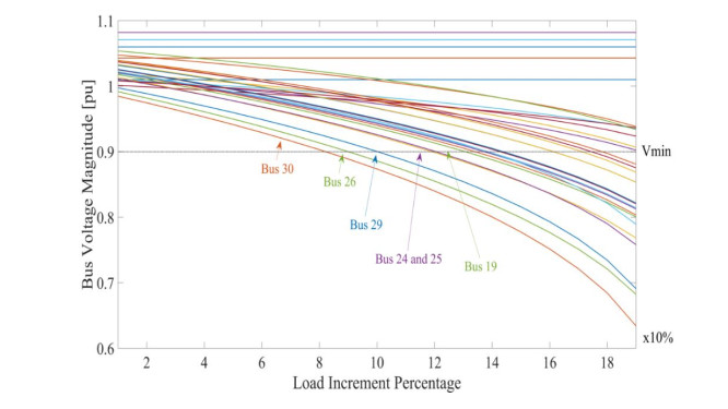
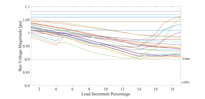
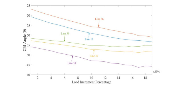
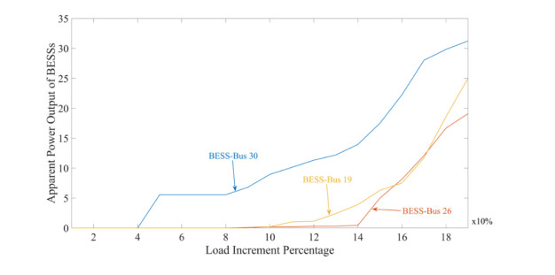
With the increase in the integration of renewable energy resources in the grid and ongoing growth in load demand worldwide, existing transmission lines are operating near their loading limits which may experience voltage collapse in a small disturbance. System stability and security can be improved when the closeness of the system to collapse is known. In this research, voltage stability of IEEE 30 bus test network is analyzed and assessed under continuously increasing load condition, utilizing the Critical Boundary Index (CBI); and improved with continuous integration of battery energy storage system (BESS). BESS is considered to be a hybrid combination of storage units and voltage source converter to have a controllable real and reactive power output. Security constraint optimal power flow is utilized for optimally sizing the installed BESS. It is evident from the outcome of the research that the voltage stability of the system is controlled to be above the acceptable range of 0.3 pu CBI in all lines and the system voltage is kept within the acceptable and constrained range of 0.9–1.1 pu.
- voltage stability,
- optimization,
- battery storage,
- transmission line,
- power control,
- genetic algorithm
Citation: Habibullah Fedayi, Mikaeel Ahmadi, Abdul Basir Faiq, Naomitsu Urasaki, Tomonobu Senjyu. BESS based voltage stability improvement enhancing the optimal control of real and reactive power compensation[J]. AIMS Energy, 2022, 10(3): 535-552. doi: 10.3934/energy.2022027

Related Papers:

Abstract

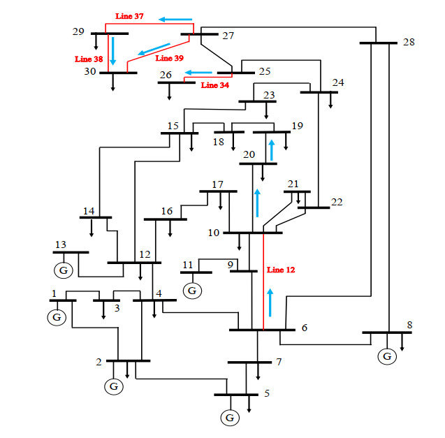
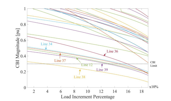
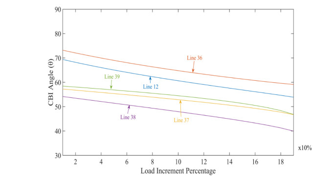
With the increase in the integration of renewable energy resources in the grid and ongoing growth in load demand worldwide, existing transmission lines are operating near their loading limits which may experience voltage collapse in a small disturbance. System stability and security can be improved when the closeness of the system to collapse is known. In this research, voltage stability of IEEE 30 bus test network is analyzed and assessed under continuously increasing load condition, utilizing the Critical Boundary Index (CBI); and improved with continuous integration of battery energy storage system (BESS). BESS is considered to be a hybrid combination of storage units and voltage source converter to have a controllable real and reactive power output. Security constraint optimal power flow is utilized for optimally sizing the installed BESS. It is evident from the outcome of the research that the voltage stability of the system is controlled to be above the acceptable range of 0.3 pu CBI in all lines and the system voltage is kept within the acceptable and constrained range of 0.9–1.1 pu.

References

[1]	Ahmadi M, Lotfy ME, Howlader AM, et al. (2019) Centralised multi-objective integration of wind farm and battery energy storage system in real-distribution network considering environmental, technical, and economic perspective. IET Gener, Trans Distrib 13: 5207-5217. https://doi.org/10.1049/iet-gtd.2018.6749 doi: 10.1049/iet-gtd.2018.6749
[2]	Ahmadi M, Lotfy ME, Danish MSS, et al. (2019) Optimal multi-configuration and allocation of SVR, capacitor, centralised wind farm, and energy storage system: a multi-objective approach in a real distribution network. IET Renewable Power Gener 13: 762-773. https://doi.org/10.1049/iet-rpg.2018.5057 doi: 10.1049/iet-rpg.2018.5057
[3]	Ahmadi M, Lotfy ME, Shigenobu R, et al. (2019) Optimal sizing of multiple renewable energy resources and PV inverter reactive power control encompassing environmental, technical, and economic issues. IEEE Syst J 13: 3026-3037. https://doi.org/10.1109/JSYST.2019.2918185 doi: 10.1109/JSYST.2019.2918185
[4]	Ahmadi M, Adewuyi OB, Danish MSS, et al. (2021) Optimum coordination of centralized and distributed renewable power generation incorporating battery storage system into the electric distribution network. Int J Electr Power Energy Syst 125: 106458. https://doi.org/10.1016/j.ijepes.2020.106458 doi: 10.1016/j.ijepes.2020.106458
[5]	Taylor CW (1994) Power System Voltage Stability, 1^st Ed., New York: McGraw-Hill, 273p.
[6]	Bode A, Shigenobu R, Ooya K, et al. (2019) Static voltage stability improvement with battery energy storage considering optimal control of active and reactive power injection. J Electr Power Syst Res 172: 303-313. https://doi.org/10.1016/j.epsr.2019.04.004 doi: 10.1016/j.epsr.2019.04.004
[7]	Canizares CA, De Souza AC, Quintana VH (1996) Comparison of performance indices for detection of proximity to voltage collapse. IEEE Trans Power Syst 11: 1441-1450. https://doi.org/10.1109/59.535685 doi: 10.1109/59.535685
[8]	Echavarren FM, Lobato E, Rouco L, et al. (2011) Formulation, computation and improvement of steady state security margins in power systems. J Electr Power Energy Syst 33: 340-346. https://doi.org/10.1016/j.ijepes.2010.08.031 doi: 10.1016/j.ijepes.2010.08.031
[9]	Mariana K, Abdelrahman AK, Ahmaed HH, et al. (2017) Development and application of a new voltage stability index for on-line monitoring and shedding. IEEE Trans Power Syst 33: 1231-1241. https://doi.org/10.1109/TPWRS.2017.2722984 doi: 10.1109/TPWRS.2017.2722984
[10]	Sayed Ali Abbas K, Dong RS (2017) DG placement in loop distribution network with new voltage stability index and loss minimization condition-based planning approach under load growth. Energies 10: 1203. https://doi.org/10.3390/en10081203 doi: 10.3390/en10081203
[11]	Moghavvemi M, Omar F (1998) Technique for contingency monitoring and voltage collapse prediciton. IEEE Proc-Gener Transm Distrib 145: 634-640. https://doi.org/10.1049/ip-gtd:19982355 doi: 10.1049/ip-gtd:19982355
[12]	Veerasamy V, Wahab NIA, Ramachandran R, et al. (2021) Recurrent network-based power flow solution for voltage stability assessment and improvement with distributed energy sources. Appl Energy 302: 117524. https://doi.org/10.1016/j.apenergy.2021.117524 doi: 10.1016/j.apenergy.2021.117524
[13]	Vadivelu KR, Marutheswar GV (2014) Fast voltage stability index based optimal reactive power planning using differential evolution. Electr Electron Eng: Int (ELELIJ) 3: 51-60.
[14]	Jirjees MA, Al-Nimma DA, Al-Hafidh MS (2018) Voltage stability enhancement based on voltage stability indices using FACTS controllers. In 2018 International Conference on Engineering Technology and their Applications (ⅡCETA), IEEE, 141-145. https://doi.org/10.1109/ⅡCETA.2018.8458094
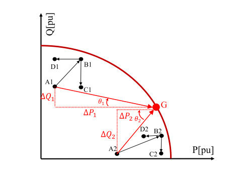
[15]	Furukakoi M, Adewuyi OB, Danish MSS, et al. (2018) Critical Boundary Index (CBI) based on active and reactive power deviations. Int J Electr Power Energy Syst 100: 50-57. https://doi.org/10.1016/j.ijepes.2018.02.010 doi: 10.1016/j.ijepes.2018.02.010
[16]	Vanishree J, Ramesh V (2014) Voltage profile improvement in power systems-A review. In 2014 International Conference on Advances in Electrical Engineering (ICAEE), IEEE, 1-4. https://doi.org/10.1109/ICAEE.2014.6838533
[17]	Leonardi B, Ajjarapu V (2012) An approach for real time voltage stability margin control via reactive power reserve sensitivities. IEEE Trans Power Syst 28: 615-625. https://doi.org/10.1109/TPWRS.2012.2212253 doi: 10.1109/TPWRS.2012.2212253
[18]	Adetokun BB, Muriithi CM (2021) Application and control of flexible alternating current transmission system devices for voltage stability enhancement of renewable-integrated power grid: A comprehensive review. Heliyon 7: e06461. https://doi.org/10.1016/j.heliyon.2021.e06461
[19]	Pradeepa H, Ananthapadmanabha T, SandhyaRani DN, et al. (2015) Optimal allocation of combined DG and capacitor units for voltage stability enhancement. Procedia Technol 21: 216-223. https://doi.org/10.1016/j.protcy.2015.10.091 doi: 10.1016/j.protcy.2015.10.091
[20]	Roselyn JP, Devaraj D, Dash SS (2014) Multi-Objective Genetic Algorithm for voltage stability enhancement using rescheduling and FACTS devices. Ain Shams Eng J 5: 789-801. https://doi.org/10.1016/j.asej.2014.04.004 doi: 10.1016/j.asej.2014.04.004
[21]	Naderi E, Narimani H, Fathi M, et al. (2017) A novel fuzzy adaptive configuration of particle swarm optimization to solve large-scale optimal reactive power dispatch. Appl Soft Comput 53: 441-456. https://doi.org/10.1016/j.asoc.2017.01.012 doi: 10.1016/j.asoc.2017.01.012
[22]	Naderi E, Pourakbari-Kasmaei M, Cerna FV, et al. (2021) A novel hybrid self-adaptive heuristic algorithm to handle single-and multi-objective optimal power flow problems. Int J Electr Power Energy Syst 125: 106492. https://doi.org/10.1016/j.ijepes.2020.106492 doi: 10.1016/j.ijepes.2020.106492
[23]	Naderi E, Pazouki S, Asrari A (2021) A region-based framework for cyberattacks leading to undervoltage in smart distribution systems. In 2021 IEEE Power and Energy Conference at Illinois (PECI), IEEE, 1-7. https://doi.org/10.1109/PECI51586.2021.9435216
[24]	Kawabe K, Yokoyama A (2014) Improvement of transient stability and short‐term voltage stability by rapid control of batteries on EHV network in power systems. Electr Eng Jpn 188: 1-10. https://doi.org/10.1002/eej.22547 doi: 10.1002/eej.22547

Reader Comments

Your name:*

Email:*
© 2022 the Author(s), licensee AIMS Press. This is an open access article distributed under the terms of the Creative Commons Attribution License (http://creativecommons.org/licenses/by/4.0)