Direct solar steam generation inside evacuated tube absorber

Khaled M. Bataineh; Assem N. AL-Karasneh; Khaled M. Bataineh; Assem N. AL-Karasneh

doi:10.3934/energy.2016.6.921

AIMS Energy

2016, Volume 4, Issue 6: 921-935. doi: 10.3934/energy.2016.6.921

Previous Article Next Article

Research article

Direct solar steam generation inside evacuated tube absorber

Department of Mechanical Engineering, Jordan University of Science and Technology, Irbid, Jordan

Received: 29 August 2016 Accepted: 01 December 2016 Published: 07 December 2016

Direct steam generation by solar radiation falling on absorber tube is studied in this paper. A system of single pipe covered by glass material in which the subcooled undergoes heating and evaporation process is analyzed. Mathematical equations are derived based on energy, momentum and mass balances for system components. A Matlab code is built to simulate the flow of water inside the absorber tube and determine properties of water along the pipe. Widely accepted empirical correlations and mathematical models of turbulent flow, pressure drop for single and multiphase flow, and heat transfer are used in the simulation. The influences of major parameters on the system performance are investigated. The pressure profiles obtained by present numerical solution for each operation condition (3 and 10 MPa) matches very well experimental data from the DISS system of Plataforma Solar de Almería. Furthermore, results obtained by simulation model for pressure profiles are closer to the experimental data than those predicted by already existed other numerical model.

Keywords:

Citation: Khaled M. Bataineh, Assem N. AL-Karasneh. Direct solar steam generation inside evacuated tube absorber[J]. AIMS Energy, 2016, 4(6): 921-935. doi: 10.3934/energy.2016.6.921

Related Papers:

[1]	Nadiyah Hussain Alharthi, Abdon Atangana, Badr S. Alkahtani . Numerical analysis of some partial differential equations with fractal-fractional derivative. AIMS Mathematics, 2023, 8(1): 2240-2256. doi: 10.3934/math.2023116
[2]	Hasib Khan, Jehad Alzabut, Anwar Shah, Sina Etemad, Shahram Rezapour, Choonkil Park . A study on the fractal-fractional tobacco smoking model. AIMS Mathematics, 2022, 7(8): 13887-13909. doi: 10.3934/math.2022767
[3]	Abdon Atangana, Seda İğret Araz . Extension of Chaplygin's existence and uniqueness method for fractal-fractional nonlinear differential equations. AIMS Mathematics, 2024, 9(3): 5763-5793. doi: 10.3934/math.2024280
[4]	Manal Alqhtani, Khaled M. Saad . Numerical solutions of space-fractional diffusion equations via the exponential decay kernel. AIMS Mathematics, 2022, 7(4): 6535-6549. doi: 10.3934/math.2022364
[5]	Abdon Atangana, Ali Akgül . Analysis of a derivative with two variable orders. AIMS Mathematics, 2022, 7(5): 7274-7293. doi: 10.3934/math.2022406
[6]	Emile Franc Doungmo Goufo, Abdon Atangana . On three dimensional fractal dynamics with fractional inputs and applications. AIMS Mathematics, 2022, 7(2): 1982-2000. doi: 10.3934/math.2022114
[7]	Rahat Zarin, Amir Khan, Pushpendra Kumar, Usa Wannasingha Humphries . Fractional-order dynamics of Chagas-HIV epidemic model with different fractional operators. AIMS Mathematics, 2022, 7(10): 18897-18924. doi: 10.3934/math.20221041
[8]	Muhammad Farman, Ali Akgül, Kottakkaran Sooppy Nisar, Dilshad Ahmad, Aqeel Ahmad, Sarfaraz Kamangar, C Ahamed Saleel . Epidemiological analysis of fractional order COVID-19 model with Mittag-Leffler kernel. AIMS Mathematics, 2022, 7(1): 756-783. doi: 10.3934/math.2022046
[9]	Amir Ali, Abid Ullah Khan, Obaid Algahtani, Sayed Saifullah . Semi-analytical and numerical computation of fractal-fractional sine-Gordon equation with non-singular kernels. AIMS Mathematics, 2022, 7(8): 14975-14990. doi: 10.3934/math.2022820
[10]	Muhammad Aslam, Muhammad Farman, Hijaz Ahmad, Tuan Nguyen Gia, Aqeel Ahmad, Sameh Askar . Fractal fractional derivative on chemistry kinetics hires problem. AIMS Mathematics, 2022, 7(1): 1155-1184. doi: 10.3934/math.2022068

Abstract

1. Introduction, definitions and preliminaries

Fractional calculus is a generalization of classical calculus and many researchers have paid attention to this science as they encounter many of these issues in the real world. Most of these issues do not have analytical exact solution. Which made many researchers interest and search in numerical and approximate methods to obtain solutions using these methods. There are many of these methods, such as the homotopy analysis ^[1,2,3,4], He's variational iteration method ^[5,6], Adomians decomposition method ^[7,8,9], Fourier spectral methods ^[10], finite difference schemes ^[11], collocation methods ^[12,13,14]. To find out more about the fractal calculus, refer to the following references ^[15,16]. More recently, a new concept was introduced for the fractional operator, as this operator has two orders, the first representing the fractional order, and the second representing the fractal dimension. In our work we aim to applied the idea of fractal-fractional derivative of orders $\beta, k$ to a reaction-diffusion equation with $q$ -th nonlinear. To this end ^[17], we replace the derivative with respect to t by the fractal-fractional derivatives power (FFP) law, the fractal-fractional exponential(FFE) law and the fractal-fractional Mittag-Leffler (FFM) law kernels which corresponds to the ^[18], Caputo-Fabrizio (CF) ^[19] and the Atangana-Baleanu (AB) ^[20] fractional derivatives, respectively. This topic has attracted many researchers and has been applied to research related to the real world, such as ^{[21,22,23,24,25,26]}. Some recent developments in the area of numerical techniques can be found in ^{[27,28,29,30,31]}.

Merkin and Needham ^[32] considered the reaction-diffusion travelling waves that can develop in a coupled system involving simple isothermal autocatalysis kinetics. They assumed that reactions took place in two separate and parallel regions, with, in $I$ , the reaction being given by quadratic autocatalysis

$\begin{equation} F + G \rightarrow 2G( \text{rate}\, k_{1}f\, g), \end{equation}$

(1.1)

together with a linear decay step

$\begin{equation} G \rightarrow H( \text{rate}\, k_{2}\, g) \end{equation}$

(1.2)

where $f$ and $g$ are the concentrations of reactant $F$ and autocatalyst $H$ , the $k_{i}(i = 1, 2)$ are the rate constants and $H$ is some inert product of reaction. The reaction in region $II$ was the quadratic autocatalytic step (1.1) only. The two regions were assumed to be coupled via a linear diffusive interchange of the autocatalytic species $G$ . We shall consider a similar system as I, but with cubic autocatalysis

$\begin{equation} F+ 2G \rightarrow 3G( \text{rate}\, k_{3}\, f g^{2}) \end{equation}$

(1.3)

together with a linear decay step

$\begin{equation} G \rightarrow H( \text{rate}\, k_{4}g). \end{equation}$

(1.4)

For $q$ -th autocatalytic, we have

$\begin{equation} F+ q G \rightarrow (q+1)G ( \text{rate} \, k_{3}f g^{q}), \, \, 1 \leq q \leq 2, \end{equation}$

(1.5)

together with a linear decay step

$\begin{equation} G \rightarrow H( \text{rate }\, k_{4} g). \end{equation}$

(1.6)

This yields to the following system

$\begin{equation} \frac{\partial \eta_{1}}{\partial t} = \frac{\partial^{2}\eta_{1}}{\partial \xi^{2}}+\nu(\eta_{2}-\eta_{1})-\eta_{1} \zeta_{1}^{q}, \end{equation}$

(1.7)

$\begin{equation} \frac{\partial \zeta_{1}}{\partial t} = \frac{\partial^{2}\zeta_{1}}{\partial \xi^{2}}-\kappa \zeta_{1}+\eta_{1} \zeta_{1}^{q}, \end{equation}$

(1.8)

$\begin{equation} \frac{\partial \eta_{2}}{\partial t} = \frac{\partial^{2}\eta_{2}}{\partial \xi^{2}}+ \nu(\eta_{1}-\eta_{2})-\eta_{2} \zeta_{2}^{q}, \end{equation}$

(1.9)

$\begin{equation} \frac{\partial \zeta_{2}}{\partial t} = \frac{\partial^{2}\zeta_{2}}{\partial \xi^{2}}+\eta_{2} \zeta_{2}^{q} \end{equation}$

(1.10)

where $\nu$ represents the couple between (I) and (II) and $\kappa$ represents the strength of the auto-catalyst decay. For more details see ^[32]. Omitting the diffusion terms in the system (1.7)-(1.10), one has the following ordinary differential equations

$\begin{equation} \frac{\partial \eta_{1}}{\partial t} = \nu(\eta_{2}-\eta_{1})-\eta_{1} \zeta_{1}^{q}, \end{equation}$

(1.11)

$\begin{equation} \frac{\partial \zeta_{1}}{\partial t} = -\kappa \zeta_{1}+\eta_{1} \zeta_{1}^{q}, \end{equation}$

(1.12)

$\begin{equation} \frac{\partial \eta_{2}}{\partial t} = \nu(\eta_{1}-\eta_{2})-\eta_{2} \zeta_{2}^{q}, \end{equation}$

(1.13)

$\begin{equation} \frac{\partial \zeta_{2}}{\partial t} = \eta_{2} \zeta_{2}^{q}. \end{equation}$

(1.14)

Now we provide some basic definitions that be needed in this work. As for the theorems and proofs related to the three fractal-fractional operators, they are found in details in ^[17]. Thus we suffice in this work by constructing the algorithms and making the numerical simulations of the set of Eqs (1.7)-(1.10) with the three fractal-fractional operators.

Definition 1. If $\eta(t)$ is continuous and fractal differentiable on $(a, b)$ of order $k$ , then the fractal-fractional derivative of $\eta(t)$ of order $\beta$ in Riemann Liouville sense with the power law is given by ^[17]:

$\begin{align} ^ \text{{FFP}}_{0}D_{t}^{\beta, \, k}\eta(t)& = \frac{1}{\Gamma(1-\beta)}\frac{d}{dt^{k}} \int_{0}^{t}(t-\tau)^{-\beta}\eta(\tau) d\tau, \, \, \, \, (0 \lt \beta, \, k \leq1), \end{align}$

(1.15)

and the fractal-fractional integral of $\eta(t)$ is given by

$\begin{align} ^{ \text{FFP}}_{\;\;\;\;\;0}{I}_t^{\beta, \, k}\eta(t) = \frac{k}{\Gamma(\beta)}\int_{0}^{t}\tau^{k-1}(t - \tau)^{\beta-1} \eta(\tau) d\tau. \end{align}$

(1.16)

Definition 2. If $\eta(t)$ is continuous in the $(a, b)$ and fractal differentiable on $(a, b)$ with order $k$ , then the fractal-fractional derivative of $\eta(t)$ of order $\beta$ in Riemann Liouville sense with the exponential decay kernel is given by ^[17]:

$\begin{align} ^{ \text{FFE}}_{0}D_{t}^{\beta, k}\eta(t)& = \frac{M(\beta)}{1-\beta}\frac{d}{dt^{k}} \int_{0}^{t} e^{\frac{-\beta}{1-\beta}(t-\tau)}\eta(\tau) d\tau, \, \, \, \, (0 \lt \beta, \, k \leq1), \end{align}$

(1.17)

and the fractal-fractional integral of $\eta(t)$ is given by

$\begin{align} ^{ \text{FFE}}_{\;\;\;\;\;0}{I}_t^{\beta, k}\eta(t) = \frac{(1-\beta) k t^{k-1}}{ M(\beta)} \eta(t)+\frac{\beta k}{M(\beta)}\int_{0}^{t}\tau^{k-1} \eta(\tau) d\tau \end{align}$

(1.18)

where $M(\beta)$ is the normalization function such that $M(0) = M(1) = 1.$

Definition 3. If $\eta(t)$ is continuous in the $(a, b)$ and fractal differentiable on $(a, b)$ with order $k$ , then the fractal-fractional derivative of $\eta(t)$ of order $\beta$ in Riemann Liouville sense with the Mittag-Leffler type kernel is given by ^[17]:

$\begin{align} ^{FFE}_{0}D_{t}^{\beta, k}\eta(t)& = \frac{A(\beta)}{1-\beta}\frac{d}{dt^{k}} \int_{0}^{t} E_{\beta}\Big({\frac{-\beta}{1-\beta}(t-\tau)}\Big)\eta(\tau) d\tau, \, \, \, \, (0 \lt \beta, \, k \leq1), \end{align}$

(1.19)

and the fractal-fractional integral of $\eta(t)$ is given by

$\begin{align} ^{ \text{FFE}}_{\;\;\;\;\;0}{I}_t^{\beta, k}\eta(t) = \frac{(1-\beta) k t^{k-1}}{ A(\beta)} \eta(t)+\frac{\beta \, k}{A(\beta) \Gamma(\beta)}\int_{0}^{t}\tau^{k-1} (t-\tau)^{\beta-1} \eta(\tau) d\tau, \end{align}$

(1.20)

$\begin{align} \frac{d\eta(t)}{dt^{k}} = lim_{\tau\rightarrow t}\frac{\eta(\tau)-\eta(t)}{\tau^{k}-t^{k}} \end{align}$

(1.21)

where where $A(\beta) = 1-\beta+\dfrac{\beta}{\Gamma(\beta)}$ is a normalization function such that $A(0) = A(1) = 1$ .

Our contribution to this paper is to construct the successive approximations and evaluate the numerical solutions of the FFRDE. These successive approximations allow us to study the behavior of numerical solutions based on power, exponential, and the Mittag-Leffler kernels. Also we can study the behavior of approximate solutions in the case of nonlinearity of the FFRDE in general. To our best knowledge, this is the first study of the FFRDE using fractal-fractional with these kernels. The importance of these results lies in the fact that they highlight the possibility of using these results for the benefit of chemical and physical researchers, by trying to link the numerical results of these mathematical models with the laboratory results. These results also contribute to the reliance on numerical results in the case of many models related to the real world, which often cannot find an analytical solution. The structure of this paper is summarized as follows: In sections, two, three and four, the FFRDE is presented with the three kernels that proposed in this work and construct the successive approximations. In section Five, numerical solutions for the FFRDE are discussed with a study of their behavior. Section Six the conclusion is presented.

2. Numerical scheme of FFRDE of q-th-order autocatalysis due the power law kernel

The new model is obtained by replacing the ordinary derivative with the the fractal-fractional derivative the power law kernel as ^[17]

$\begin{align} ^{ \text{FFP}}_{0}D_{t}^{\beta}\eta_{1}(t) = \nu(\eta_{2}(t)-\eta_{1}(t))-\eta_{1}(t) \zeta_{1}^{q}(t), \end{align}$

(2.1)

$\begin{align} ^{ \text{FFP}}_{0}D_{t}^{\beta}\zeta_{1}(t) = -\kappa \zeta_{1}(t)+\eta_{1}(t) \zeta_{1}^{q}(t), \end{align}$

(2.2)

$\begin{align} ^{ \text{FFP}}_{0}D_{t}^{\beta}\eta_{2}(t) = \nu(\eta_{1}(t)-\eta_{2}(t))-\eta_{2}(t) \zeta_{2}^{q}(t), \end{align}$

(2.3)

$\begin{align} ^{ \text{FFP}}_{0}D_{t}^{\beta}\zeta_{2}(t) = \eta_{2}(t) \zeta_{2}^{q}(t). \end{align}$

(2.4)

By following the procedure in ^[17], we can obtain the following successive approximations:

$\begin{align} \eta_{1}(t) - \eta_{1}(0) & = \frac{k}{\Gamma(\beta)} \int_{0}^{t} \tau^{k-1} (t - \tau)^{\beta - 1} \varphi_{1}(\eta_{1}, \zeta_{1}, \eta_{2}, \zeta_{2}, \tau)d\tau, \end{align}$

(2.5)

$\begin{align} \zeta_{1}(t) - \zeta_{2}(0) & = \frac{k}{\Gamma(\beta)} \int_{0}^{t} \tau^{k-1} (t - \tau)^{\beta - 1} \varphi_{2}(\eta_{1}, \zeta_{1}, \eta_{2}, \zeta_{2}, \tau)d\tau, \end{align}$

(2.6)

$\begin{align} \eta_{2}(t) - \eta_{3}(0) & = \frac{k}{\Gamma(\beta)} \int_{0}^{t} \tau^{k-1}(t - \tau)^{\beta - 1} \varphi_{3}(\eta_{1}, \zeta_{1}, \eta_{2}, \zeta_{2}, \tau)d\tau, \end{align}$

(2.7)

$\begin{align} \zeta_{2}(t) - \zeta_{2}(0) & = \frac{k}{\Gamma(\beta)} \int_{0}^{t} \tau^{k-1} (t - \tau)^{\beta - 1}\varphi_{4}(\eta_{1}, \zeta_{1}, \eta_{2}, \zeta_{2}, \tau) d\tau \end{align}$

(2.8)

where

$\begin{align} \varphi_{1}(\eta_{1}, \zeta_{1}, \eta_{2}, \zeta_{2}, \tau)& = \Big(\nu\, (\eta_{2}(\tau)-\eta_{1}(\tau))-\eta_{1}(\tau) \zeta_{1}^{q}(\tau)\Big), \end{align}$

(2.9)

$\begin{align} \varphi_{2}(\eta_{1}, \zeta_{1}, \eta_{2}, \zeta_{2}, \tau)& = \Big( -\kappa \, \zeta_{1}(\tau)+\eta_{1}(\tau) \zeta_{1}^{q}(\tau)\Big), \end{align}$

(2.10)

$\begin{align} \varphi_{3}(\eta_{1}, \zeta_{1}, \eta_{2}, \zeta_{2}, \tau)& = \Big(\nu(\eta_{1}(\tau)-\eta_{2}(\tau))-\eta_{2}(\tau) \zeta_{2}^{q}(\tau)\Big), \end{align}$

(2.11)

$\begin{align} \varphi_{4}(\eta_{1}, \zeta_{1}, \eta_{2}, \zeta_{2}, \tau)& = \eta_{2}(\tau) \zeta_{2}^{q}(\tau). \end{align}$

(2.12)

Equation (2.5)-(2.8) can be reformulated as

$\begin{equation} \eta_{1}(t) - \eta_{1}(0) = \frac{k}{\Gamma(\beta)}\sum\limits_{m = 0}^{n} \int_{t_{m}}^{t_{m+1}} \tau^{k-1} (t_{n+1} - \tau)^{\beta - 1} \varphi_{1}(\eta_{1}, \zeta_{1}, \eta_{2}, \zeta_{2}, \tau)d\tau, \end{equation}$

(2.13)

$\begin{equation} \zeta_{1}(t) - \zeta_{1}(0) = \frac{k}{\Gamma(\beta)}\sum\limits_{m = 0}^{n} \int_{t_{m}}^{t_{m+1}} \tau^{k-1} (t_{n+1} - \tau)^{\beta - 1} \varphi_{2}(\eta_{1}(\tau), \zeta_{1}(\tau), \eta_{2}(\tau), \zeta_{2}(\tau), \tau)d\tau, \end{equation}$

(2.14)

$\begin{equation} \eta_{2}(t) - \eta_{2}(0) = \frac{k}{\Gamma(\beta)} \sum\limits_{m = 0}^{n} \int_{t_{m}}^{t_{m+1}} \tau^{k-1}(t_{n+1} - \tau)^{\beta - 1} \varphi_{3}(\eta_{1}, \zeta_{1}, \eta_{2}, \zeta_{2}, \tau)d\tau, \end{equation}$

(2.15)

$\begin{equation} \zeta_{2}(t) - \zeta_{2}(0) = \frac{k}{\Gamma(\beta)} \sum\limits_{m = 0}^{n} \int_{t_{m}}^{t_{m+1}} \tau^{k-1} (t_{n+1} - \tau)^{\beta - 1}\varphi_{4}(\eta_{1}, \zeta_{1}, \eta_{2}, \zeta_{2}, \tau)d\tau. \end{equation}$

(2.16)

Using the two-step Lagrange polynomial interpolation, we obtain

$\begin{align} \eta_{1}(t) - \eta_{1}(0) & = \frac{k}{\Gamma(\beta)}\sum\limits_{m = 0}^{n} \int_{t_{m}}^{t_{m+1}} (t_{n+1} - \tau)^{\beta - 1} Q_{1, m}(\tau)d\tau, \end{align}$

(2.17)

$\begin{align} \zeta_{1}(t) - \zeta_{1}(0) & = \frac{k}{\Gamma(\beta)}\sum\limits_{m = 0}^{n} \int_{t_{m}}^{t_{m+1}} (t_{n+1} - \tau)^{\beta - 1} Q_{2, m}(\tau)d\tau, \end{align}$

(2.18)

$\begin{align} \eta_{2}(t) - \eta_{2}(0) & = \frac{k}{\Gamma(\beta)} \sum\limits_{m = 0}^{n} \int_{t_{m}}^{t_{m+1}} (t_{n+1} - \tau)^{\beta - 1}Q_{3, m}(\tau)d\tau, \end{align}$

(2.19)

$\begin{align} \zeta_{2}(t) - \zeta_{2}(0) & = \frac{k}{\Gamma(\beta)} \sum\limits_{m = 0}^{n} \int_{t_{m}}^{t_{m+1}} (t_{n+1} - \tau)^{\beta - 1}Q_{4, m}(\tau) d\tau, \end{align}$

(2.20)

where,

$\begin{align} Q_{1, m}(\tau)& = \frac{\tau-t_{m-1}}{t_{m}-t_{m-1}}t^{k-1}_{m}\varphi_{1}(\eta_{1}(\tau_{m}), \zeta_{1}(\tau_{m}), \eta_{2}(\tau_{m}), \zeta_{2}(\tau_{m}), \tau_{m})-\frac{\tau-t_{m}}{t_{m}-t_{m-1}}\\ \times&t^{k-1}_{m-1}\varphi_{1}(\eta_{1}(\tau_{m-1}), \zeta_{1}(\tau_{m-1}), \eta_{2}(\tau_{m-1}), \zeta_{2}(\tau_{m-1}), \tau_{m-1}), \end{align}$

(2.21)

$\begin{align} Q_{2, m}(\tau)& = \frac{\tau-t_{m-1}}{t_{m}-t_{m-1}}t^{k-1}_{m}\varphi_{2}(\eta_{1}(\tau_{m}), \zeta_{1}(\tau_{m}), \eta_{2}(\tau_{m}), \zeta_{2}(\tau_{m}), \tau_{m})-\frac{\tau-t_{m}}{t_{m}-t_{m-1}}\\ \times&t^{k-1}_{m-1}\varphi_{2}(\eta_{1}(\tau_{m-1}), \zeta_{1}(\tau_{m-1}), \eta_{2}(\tau_{m-1}), \zeta_{2}(\tau_{m-1}), \tau_{m-1}), \end{align}$

(2.22)

$\begin{align} Q_{3, m}(\tau)& = \frac{\tau-t_{m-1}}{t_{m}-t_{m-1}}t^{k-1}_{m}\varphi_{3}(\eta_{1}(\tau_{m}), \zeta_{1}(\tau_{m}), \eta_{2}(\tau_{m}), \zeta_{2}(\tau_{m}), \tau_{m})-\frac{\tau-t_{m}}{t_{m}-t_{m-1}}\\ \times&t^{k-1}_{m-1}\varphi_{3}(\eta_{1}(\tau_{m-1}), \zeta_{1}(\tau_{m-1}), \eta_{2}(\tau_{m-1}), \zeta_{2}(\tau_{m-1}), \tau_{m-1}), \end{align}$

(2.23)

$\begin{align} Q_{4, m}(\tau)& = \frac{\tau-t_{m-1}}{t_{m}-t_{m-1}}t^{k-1}_{m}\varphi_{4}(\eta_{4}(\tau_{m}), \zeta_{1}(\tau_{m}), \eta_{2}(\tau_{m}), \zeta_{2}(\tau_{m}), \tau_{m})-\frac{\tau-t_{m}}{t_{m}-t_{m-1}}\\ \times&t^{k-1}_{m-1}\varphi_{4}(\eta_{1}(\tau_{m-1}), \zeta_{1}(\tau_{m-1}), \eta_{2}(\tau_{m-1}), \zeta_{2}(\tau_{m-1}), \tau_{m-1}). \end{align}$

(2.24)

These integrals are evaluated directly and the numerical solutions of (2.1)-(2.4) involving the FFP derivative are given by

$\begin{eqnarray} \eta_{1}(t_{n+1}) & = & \eta_{1}(0) + \frac{k h^{\beta}}{\Gamma(\beta+2)} \sum\limits_{m = 0}^{n} t^{k-1}_{m} \varphi_{1}(\eta_{1}(t_{m}), \zeta_{1}(t_{m}), \eta_{2}(t_{m}), \zeta_{2}(t_{m}), t_{m})\Xi_{1}(n, m) \\ &-&t^{k-1}_{m-1}\varphi_{1}(\eta_{1}(\tau_{m-1}), \zeta_{1}(t_{m-1}), \eta_{2}(t_{m-1}), \zeta_{2}(t_{m-1}), t_{m-1})\Xi_{2}(n, m)\Big), \end{eqnarray}$

(2.25)

$\begin{eqnarray} \zeta_{1}(t_{n+1}) & = & \zeta_{1}(0) + \frac{k h^{\beta}}{\Gamma(\beta+2)} \sum\limits_{m = 0}^{n} t^{k-1}_{m} \varphi_{2}(\eta_{1}(t_{m}), \zeta_{1}(t_{m}), \eta_{2}(t_{m}), \zeta_{2}(t_{m}), t_{m})\Xi_{1}(n, m) \\ &-&t^{k-1}_{m-1}\varphi_{2}(\eta_{1}(\tau_{m-1}), \zeta_{1}(t_{m-1}), \eta_{2}(t_{m-1}), \zeta_{2}(t_{m-1}), t_{m-1})\Xi_{2}(n, m)\Big), \end{eqnarray}$

(2.26)

$\begin{eqnarray} \eta_{2}(t_{n+1}) & = & \eta_{2}(0) + \frac{k h^{\beta}}{\Gamma(\beta+2)} \sum\limits_{m = 0}^{n} t^{k-1}_{m} \varphi_{3}(\eta_{1}(t_{m}), \zeta_{1}(t_{m}), \eta_{2}(t_{m}), \zeta_{2}(t_{m}), t_{m})\Xi_{1}(n, m) \\ &-&t^{k-1}_{m-1}\varphi_{4}(\eta_{1}(\tau_{m-1}), \zeta_{1}(t_{m-1}), \eta_{2}(t_{m-1}), \zeta_{2}(t_{m-1}), t_{m-1})\Xi_{2}(n, m)\Big), \end{eqnarray}$

(2.27)

$\begin{eqnarray} \zeta_{2}(t_{n+1}) & = & \zeta_{2}(0) + \frac{k h^{\beta}}{\Gamma(\beta+2)} \sum\limits_{m = 0}^{n} t^{k-1}_{m} \varphi_{4}(\eta_{1}(t_{m}), \zeta_{1}(t_{m}), \eta_{2}(t_{m}), \zeta_{2}(t_{m}), t_{m})\Xi_{1}(n, m) \\ &-&t^{k-1}_{m-1}\varphi_{4}(\eta_{1}(\tau_{m-1}), \zeta_{1}(t_{m-1}), \eta_{2}(t_{m-1}), \zeta_{2}(t_{m-1}), t_{m-1})\Xi_{2}(n, m)\Big), \end{eqnarray}$

(2.28)

$\begin{equation} \begin{aligned} \Xi_{1}(n, m)& = \Big((n + 1 - m)^{\beta}(n -m + 2 + \beta) - (n - m)^{\beta}\times (n -m + 2 + 2\beta) \Big), \end{aligned} \end{equation}$

(2.29)

$\begin{equation} \begin{aligned} \Xi_{2}(n, m) = \Big((n + 1 - m)^{\beta+1} - (n -m)^{\beta}(n -m + 1 + \beta)\Big). \end{aligned} \end{equation}$

(2.30)

3. Numerical scheme of FFRDE of $q$ -th-order autocatalysis due the exponential decay kernel

Considering the FFE derivative, we have from ^[17]

$\begin{align} ^{ \text{FFE}}_{0}D_{t}^{\beta}\eta_{1}(t) = \nu(\eta_{2}(t)-\eta_{1}(t))-\eta_{1}(t) \zeta_{1}^{q}(t), \end{align}$

(3.1)

$\begin{align} ^{ \text{FFE}}_{0}D_{t}^{\beta}\zeta_{1}(t) = -\kappa \zeta_{1}(t)+\eta_{1}(t) \zeta_{1}^{q}(t), \end{align}$

(3.2)

$\begin{align} ^{ \text{FFE}}_{0}D_{t}^{\beta}\eta_{2}(t) = \nu(\eta_{1}(t)-\eta_{2}(t))-\eta_{2}(t) \zeta_{2}^{q}(t), \end{align}$

(3.3)

$\begin{align} ^{ \text{FFE}}_{0}D_{t}^{\beta}\zeta_{2}(t) = \eta_{2}(t) \zeta_{2}^{q}(t). \end{align}$

(3.4)

For the successive approximations of the system (3.1)-(3.4), we follow the same procedures as in ^[17], we obtain

$\begin{eqnarray} \eta_{1}(t)- \eta_{1}(0) & = & \frac{k t^{k-1}(1 - \beta)}{M(\beta)} \varphi_{1}(\eta_{1}, \zeta_{1}, \eta_{2}, \zeta_{2}, t) \\ &+& \frac{\beta}{M(\beta)} \int_{0}^{t} k\, \tau^{k-1}\varphi_{1}(\eta_{1}, \zeta_{1}, \eta_{2}, \zeta_{2}, \tau) d\tau, \end{eqnarray}$

(3.5)

$\begin{eqnarray} \zeta_{1}(t)- \zeta_{1}(0) & = & \frac{k t^{k-1}(1 - \beta)}{M(\beta)} \varphi_{2}(\eta_{1}, \zeta_{1}, \eta_{2}, \zeta_{2}, t) \\ &+& \frac{\beta}{M(\beta)} \int_{0}^{t} k\, \tau^{k-1}\varphi_{2}(\eta_{1}, \zeta_{1}, \eta_{2}, \zeta_{2}, \tau) d\tau, \end{eqnarray}$

(3.6)

$\begin{eqnarray} \eta_{2}(t)- \eta_{2}(0) & = & \frac{k t^{k-1}(1 - \beta)}{M(\beta)} \varphi_{3}(\eta_{1}, \zeta_{1}, \eta_{2}, \zeta_{2}, t) \\ &+& \frac{\beta}{M(\beta)} \int_{0}^{t} k\, \tau^{k-1}\varphi_{3}(\eta_{1}, \zeta_{1}, \eta_{2}, \zeta_{2}, \tau) d\tau, \end{eqnarray}$

(3.7)

$\begin{eqnarray} \zeta_{2}(t)- \zeta_{2}(0) & = & \frac{k t^{k-1}(1 - \beta)}{M(\beta)} \varphi_{4}(\eta_{1}, \zeta_{1}, \eta_{2}, \zeta_{2}, t) \\ &+& \frac{\beta}{M(\beta)} \int_{0}^{t} k\, \tau^{k-1}\varphi_{4}(\eta_{1}, \zeta_{1}, \eta_{2}, \zeta_{2}, \tau) d\tau. \end{eqnarray}$

(3.8)

Using $t = t_{n+1}$ the following is established

$\begin{eqnarray} \eta_{1}(t_{n+1})- \eta_{1}(0) & = & \frac{k t^{k-1}(1 - \beta)}{M(\beta)} \varphi_{1}(\eta_{1}, \zeta_{1}, \eta_{2}, \zeta_{2}, t_{n}) \\ &+& \frac{\beta}{M(\beta)} \int_{0}^{t_{n+1}} k\, \tau^{k-1}\varphi_{1}(\eta_{1}, \zeta_{1}, \eta_{2}, \zeta_{2}, \tau) d\tau, \end{eqnarray}$

(3.9)

$\begin{eqnarray} \zeta_{1}(t_{n+1})- \zeta_{1}(0) & = & \frac{k t^{k-1}(1 - \beta)}{M(\beta)} \varphi_{2}(\eta_{1}, \zeta_{1}, \eta_{2}, \zeta_{2}, t_{n}) \\ &+& \frac{\beta}{M(\beta)} \int_{0}^{t_{n+1}} k\, \tau^{k-1}\varphi_{2}(\eta_{1}, \zeta_{1}, \eta_{2}, \zeta_{2}, \tau) d\tau, \end{eqnarray}$

(3.10)

$\begin{eqnarray} \eta_{2}(t_{n+1})- \eta_{2}(0) & = & \frac{k t^{k-1}(1 - \beta)}{M(\beta)} \varphi_{3}(\eta_{1}, \zeta_{1}, \eta_{2}, \zeta_{2}, t_{n}) \\ &+& \frac{\beta}{M(\beta)} \int_{0}^{t_{n+1}} k\, \tau^{k-1}\varphi_{3}(\eta_{1}, \zeta_{1}, \eta_{2}, \zeta_{2}, \tau) d\tau, \end{eqnarray}$

(3.11)

$\begin{eqnarray} \zeta_{2}(t_{n+1})- \zeta_{2}(0) & = & \frac{k t^{k-1}(1 - \beta)}{M(\beta)} \varphi_{4}(\eta_{1}, \zeta_{1}, \eta_{2}, \zeta_{2}, t_{n}) \\ &+& \frac{\beta}{M(\beta)} \int_{0}^{t_{n+1}} k\, \tau^{k-1}\varphi_{4}(\eta_{1}, \zeta_{1}, \eta_{2}, \zeta_{2}, \tau) d\tau. \end{eqnarray}$

(3.12)

Further, we have the following:

$\begin{eqnarray} \eta_{1}(t_{n+1})- \eta_{1}(t_{n}) & = & \frac{k t^{k-1}_{n}(1 - \beta)}{M(\beta)} \varphi_{1}(\eta_{1}, \zeta_{1}, \eta_{2}, \zeta_{2}, t_{n}) \\ &-&\frac{k t^{k-1}_{n-1}(1 - \beta)}{M(\beta)}\varphi_{1}(\eta_{1}, \zeta_{1}, \eta_{2}, \zeta_{2}, t_{n-1}) \\ &+& \frac{\beta}{M(\beta)} \int_{t_{n}}^{t_{n+1}} k\, \tau^{k-1}\varphi_{1}(\eta_{1}, \zeta_{1}, \eta_{2}, \zeta_{2}, \tau) d\tau, \end{eqnarray}$

(3.13)

$\begin{eqnarray} \zeta_{1}(t_{n+1})- \zeta_{1}(t_{n}) & = & \frac{k t^{k-1}_{n}(1 - \beta)}{M(\beta)} \varphi_{2}(\eta_{1}, \zeta_{1}, \eta_{2}, \zeta_{2}, t_{n}) \\ &-&\frac{k t^{k-1}_{n-1}(1 - \beta)}{M(\beta)}\varphi_{2}(\eta_{1}, \zeta_{1}, \eta_{2}, \zeta_{2}, t_{n-1}) \\ &+& \frac{\beta}{M(\beta)} \int_{t_{n}}^{t_{n+1}} k\, \tau^{k-1}\varphi_{2}(\eta_{1}, \zeta_{1}, \eta_{2}, \zeta_{2}, \tau) d\tau, \end{eqnarray}$

(3.14)

$\begin{eqnarray} \eta_{2}(t_{n+1})- \eta_{2}(t_{n}) & = & \frac{k t^{k-1}_{n}(1 - \beta)}{M(\beta)} \varphi_{3}(\eta_{1}, \zeta_{1}, \eta_{2}, \zeta_{2}, t_{n}) \\ &-&\frac{k t^{k-1}_{n-1}(1 - \beta)}{M(\beta)}\varphi_{3}(\eta_{1}, \zeta_{1}, \eta_{2}, \zeta_{2}, t_{n-1}) \\ &+& \frac{\beta}{M(\beta)} \int_{t_{n}}^{t_{n+1}} k\, \tau^{k-1}\varphi_{3}(\eta_{1}, \zeta_{1}, \eta_{2}, \zeta_{2}, \tau) d\tau, \end{eqnarray}$

(3.15)

$\begin{eqnarray} \zeta_{2}(t_{n+1})- \zeta_{2}(t_{n}) & = & \frac{k t^{k-1}_{n}(1 - \beta)}{M(\beta)} \varphi_{4}(\eta_{1}, \zeta_{1}, \eta_{2}, \zeta_{2}, t_{n}) \\ &-&\frac{k t^{k-1}_{n-1}(1 - \beta)}{M(\beta)}\varphi_{4}(\eta_{1}, \zeta_{1}, \eta_{2}, \zeta_{2}, t_{n-1}) \\ &+& \frac{\beta}{M(\beta)} \int_{t_{n}}^{t_{n+1}} k\, \tau^{k-1}\varphi_{4}(\eta_{1}, \zeta_{1}, \eta_{2}, \zeta_{2}, \tau) d\tau. \end{eqnarray}$

(3.16)

It follows from the Lagrange polynomial interpolation and integrating the following expressions:

$\begin{eqnarray} \eta_{1}(t_{n+1})- \eta_{1}(t_{n}) & = & \frac{k t^{k-1}_{n}(1 - \beta)}{M(\beta)} \varphi_{1}(\eta_{1}, \zeta_{1}, \eta_{2}, \zeta_{2}, t_{n}) \\ &-&\frac{k t^{k-1}_{n-1}(1 -\beta)}{M(\beta)} \varphi_{1}(\eta_{1}, \zeta_{1}, \eta_{2}, \zeta_{2}, t_{n-1}) +\frac{k h \beta }{2 M(\beta)} \\ &\times& \Big(3 t^{k-1}_{n}\varphi_{1}(\eta_{1}, \zeta_{1}, \eta_{2}, \zeta_{2}, t_{n}) -t^{k-1}_{n-1}\varphi_{1}(\eta_{1}, \zeta_{1}, \eta_{2}, \zeta_{2}, t_{n-1}) , \end{eqnarray}$

(3.17)

$\begin{eqnarray} \zeta_{1}(t_{n+1})- \zeta_{1}(t_{n}) & = & \frac{k t^{k-1}_{n}(1 - \beta)}{M(\beta)} \varphi_{2}(\eta_{1}, \zeta_{1}, \eta_{2}, \zeta_{2}, t_{n}) \\ &-&\frac{k t^{k-1}_{n-1}(1 -\beta)}{M(\beta)} \varphi_{2}(\eta_{1}, \zeta_{1}, \eta_{2}, \zeta_{2}, t_{n-1}) +\frac{k h \beta }{2 M(\beta)} \\ &\times& \Big(3 t^{k-1}_{n}\varphi_{2}(\eta_{1}, \zeta_{1}, \eta_{2}, \zeta_{2}, t_{n}) -t^{k-1}_{n-1}\varphi_{2}(\eta_{1}, \zeta_{1}, \eta_{2}, \zeta_{2}, t_{n-1}) , \end{eqnarray}$

(3.18)

$\begin{eqnarray} \eta_{2}(t_{n+1})- \eta_{2}(t_{n}) & = & \frac{k t^{k-1}_{n}(1 - \beta)}{M(\beta)} \varphi_{3}(\eta_{1}, \zeta_{1}, \eta_{2}, \zeta_{2}, t_{n}) \\ &-&\frac{k t^{k-1}_{n-1}(1 -\beta)}{M(\beta)} \varphi_{3}(\eta_{1}, \zeta_{1}, \eta_{2}, \zeta_{2}, t_{n-1}) +\frac{k h \beta }{2 M(\beta)} \\ &\times& \Big(3 t^{k-1}_{n}\varphi_{3}(\eta_{1}, \zeta_{1}, \eta_{2}, \zeta_{2}, t_{n}) -t^{k-1}_{n-1}\varphi_{3}(\eta_{1}, \zeta_{1}, \eta_{2}, \zeta_{2}, t_{n-1}) , \end{eqnarray}$

(3.19)

$\begin{eqnarray} \zeta_{2}(t_{n+1})- \zeta_{2}(t_{n}) & = & \frac{k t^{k-1}_{n}(1 - \beta)}{M(\beta)} \varphi_{4}(\eta_{1}, \zeta_{1}, \eta_{2}, \zeta_{2}, t_{n}) \\ &-&\frac{k t^{k-1}_{n-1}(1 -\beta)}{M(\beta)} \varphi_{4}(\eta_{1}, \zeta_{1}, \eta_{2}, \zeta_{2}, t_{n-1}) +\frac{k h \beta }{2 M(\beta)} \\ &\times& \Big(3 t^{k-1}_{n}\varphi_{4}(\eta_{1}, \zeta_{1}, \eta_{2}, \zeta_{2}, t_{n}) -t^{k-1}_{n-1}\varphi_{4}(\eta_{1}, \zeta_{1}, \eta_{2}, \zeta_{2}, t_{n-1}). \end{eqnarray}$

(3.20)

Finally, it is appropriate to write the successive approximations of the system (3.1)-(3.4) as follows:

$\begin{eqnarray} \eta_{1}(t_{n+1})- \eta_{1}(t_{n}) & = & k t^{k-1}_{n} \Big(\frac{(1 - \beta)}{M(\beta)}+\frac{3h\beta}{2 M(\beta)}\Big) \varphi_{1}(\eta_{1}, \zeta_{1}, \eta_{2}, \zeta_{2}, t_{n}) \\ &-& k t^{k-1}_{n-1} \Big(\frac{(1 - \beta)}{M(\beta)}+\frac{h\beta}{2 M(\beta)}\Big) \varphi_{1}(\eta_{1}, \zeta_{1}, \eta_{2}, \zeta_{2}, t_{n-1}), \end{eqnarray}$

(3.21)

$\begin{eqnarray} \zeta_{1}(t_{n+1})-\zeta_{1}(t_{n}) & = & k t^{k-1}_{n} \Big(\frac{(1 - \beta)}{M(\beta)}+\frac{3h\beta}{2 M(\beta)}\Big) \varphi_{2}(\eta_{1}, \zeta_{1}, \eta_{2}, \zeta_{2}, t_{n}) \\ &-& k t^{k-1}_{n-1} \Big(\frac{(1 - \beta)}{M(\beta)}+\frac{h\beta}{2 M(\beta)}\Big) \varphi_{2}(\eta_{1}, \zeta_{1}, \eta_{2}, \zeta_{2}, t_{n-1}), \end{eqnarray}$

(3.22)

$\begin{eqnarray} \eta_{2}(t_{n+1})- \eta_{2}(t_{n}) & = & k t^{k-1}_{n} \Big(\frac{(1 - \beta)}{M(\beta)}+\frac{3h\beta}{2 M(\beta)}\Big) \varphi_{3}(\eta_{1}, \zeta_{1}, \eta_{2}, \zeta_{2}, t_{n}) \\ &-& k t^{k-1}_{n-1} \Big(\frac{(1 - \beta)}{M(\beta)}+\frac{h\beta}{2 M(\beta)}\Big) \varphi_{3}(\eta_{1}, \zeta_{1}, \eta_{2}, \zeta_{2}, t_{n-1}), \end{eqnarray}$

(3.23)

$\begin{eqnarray} \zeta_{2}(t_{n+1})-\zeta_{2}(t_{n}) & = & k t^{k-1}_{n} \Big(\frac{(1 - \beta)}{M(\beta)}+\frac{3h\beta}{2 M(\beta)}\Big) \varphi_{4}(\eta_{1}, \zeta_{1}, \eta_{2}, \zeta_{2}, t_{n}) \\ &-& k t^{k-1}_{n-1} \Big(\frac{(1 - \beta)}{M(\beta)}+\frac{h\beta}{2 M(\beta)}\Big) \varphi_{4}(\eta_{1}, \zeta_{1}, \eta_{2}, \zeta_{2}, t_{n-1}). \end{eqnarray}$

(3.24)

4. Numerical scheme of FFRDE of $q$ -th-order autocatalysis due the generalized Mittag Lefller kernel

Considering the FFM derivative, we have ^[18]

$\begin{align} ^{ \text{FFM}}_{0}D_{t}^{\beta}\eta_{1}(t) = \nu(\eta_{2}(t)-\eta_{1}(t))-\eta_{1}(t) \zeta_{1}^{q}(t), \end{align}$

(4.1)

$\begin{align} ^{ \text{FFM}}_{0}D_{t}^{\beta}\zeta_{1}(t) = -\kappa \zeta_{1}(t)+\eta_{1}(t) \zeta_{1}^{q}(t), \end{align}$

(4.2)

$\begin{align} ^{ \text{FFM}}_{0}D_{t}^{\beta}\eta_{2}(t) = \nu(\eta_{1}(t)-\eta_{2}(t))-\eta_{2}(t) \zeta_{2}^{q}(t), \end{align}$

(4.3)

$\begin{align} ^{ \text{FFM}}_{0}D_{t}^{\beta}\zeta_{2}(t) = \eta_{2}(t) \zeta_{2}^{q}(t). \end{align}$

(4.4)

Also, for this system (4.1)-(4.4), we follow the same treatment that was done in ^[17] to obtain the successive approximate solutions as follows:

$\begin{eqnarray} \eta_{1}(t)- \eta_{1}(0) & = & \frac{k t^{k-1}(1 - \beta)}{A(\beta)} \varphi_{1}(\eta_{1}, \zeta_{1}, \eta_{2}, \zeta_{2}, t) \\ &+& \frac{\beta}{A(\beta) \Gamma(\beta)} \int_{0}^{t} k\, \tau^{k-1}(t-\tau)^{\beta-1} \varphi_{1}(\eta_{1}, \zeta_{1}, \eta_{2}, \zeta_{2}, \tau) d\tau, \end{eqnarray}$

(4.5)

$\begin{eqnarray} \zeta_{1}(t)- \zeta_{1}(0) & = & \frac{k t^{k-1}(1 - \beta)}{A(\beta)} \varphi_{2}(\eta_{1}, \zeta_{1}, \eta_{2}, \zeta_{2}, t) \\ &+& \frac{\beta}{A(\beta) \Gamma(\beta)} \int_{0}^{t} k\, \tau^{k-1} (t-\tau)^{\beta-1}\varphi_{2}(\eta_{1}, \zeta_{1}, \eta_{2}, \zeta_{2}, \tau) d\tau, \end{eqnarray}$

(4.6)

$\begin{eqnarray} \eta_{2}(t)- \eta_{2}(0) & = & \frac{k t^{k-1}(1 - \beta)}{A(\beta)} \varphi_{3}(\eta_{1}, \zeta_{1}, \eta_{2}, \zeta_{2}, t) \\ &+& \frac{\beta}{A(\beta) \Gamma(\beta)} \int_{0}^{t} k\, \tau^{k-1} (t-\tau)^{\beta-1}\varphi_{3}(\eta_{1}, \zeta_{1}, \eta_{2}, \zeta_{2}, \tau) d\tau, \end{eqnarray}$

(4.7)

$\begin{eqnarray} \zeta_{2}(t)- \zeta_{2}(0) & = & \frac{k t^{k-1}(1 - \beta)}{A(\beta)} \varphi_{4}(\eta_{1}, \zeta_{1}, \eta_{2}, \zeta_{2}, t) \\ &+& \frac{\beta}{A(\beta) \Gamma(\beta)} \int_{0}^{t} k\, \tau^{k-1} (t-\tau)^{\beta-1}\varphi_{4}(\eta_{1}, \zeta_{1}, \eta_{2}, \zeta_{2}, \tau) d\tau. \end{eqnarray}$

(4.8)

At $t_{n+1}$ we obtain the following

(4.9)

(4.10)

(4.11)

(4.12)

The integrals involving in (4.9)-(4.12) can be approximated as:

$\begin{eqnarray} \eta_{1}(t_{n+1})- \eta_{1}(0) & = & \frac{k t_{n}^{k-1}(1 - \beta)}{A(\beta)} \varphi_{1}(\eta_{1}(t_{n}), \zeta_{1}(t_{n}), \eta_{2}(t_{n}), \zeta_{2}(t_{n}), t_{n}) \\ &+& \frac{\beta}{A(\beta) \Gamma(\beta)} \sum\limits_{m = 0}^{n}\int_{t_{m}}^{t_{m+1}} k\, \tau^{k-1}(t_{n+1}-\tau)^{\beta-1} \varphi_{1}(\eta_{1}, \zeta_{1}, \eta_{2}, \zeta_{2}, \tau) d\tau, \end{eqnarray}$

(4.13)

$\begin{eqnarray} \zeta_{1}(t_{n+1})- \zeta_{1}(0) & = & \frac{k t_{n}^{k-1}(1 - \beta)}{A(\beta)} \varphi_{2}(\eta_{1}(t_{n}), \zeta_{1}(t_{n}), \eta_{2}(t_{n}), \zeta_{2}(t_{n}), t_{n}) \\ &+& \frac{\beta}{A(\beta) \Gamma(\beta)} \sum\limits_{m = 0}^{n}\int_{t_{m}}^{t_{m+1}} k\, \tau^{k-1} (t_{n+1}-\tau)^{\beta-1}\varphi_{2}(\eta_{1}, \zeta_{1}, \eta_{2}, \zeta_{2}, \tau) d\tau, \end{eqnarray}$

(4.14)

$\begin{eqnarray} \eta_{2}(t_{n+1})- \eta_{2}(0) & = & \frac{k t_{n}^{k-1}(1 - \beta)}{A(\beta)} \varphi_{3}(\eta_{1}(t_{n}), \zeta_{1}(t_{n}), \eta_{2}(t_{n}), \zeta_{2}(t_{n}), t_{n}) \\ &+& \frac{\beta}{A(\beta) \Gamma(\beta)} \sum\limits_{m = 0}^{n}\int_{t_{m}}^{t_{m+1}} k\, \tau^{k-1} (t_{n+1}-\tau)^{\beta-1}\varphi_{3}(\eta_{1}, \zeta_{1}, \eta_{2}, \zeta_{2}, \tau) d\tau, \end{eqnarray}$

(4.15)

$\begin{eqnarray} \zeta_{2}(t_{n+1})- \zeta_{2}(0) & = & \frac{k t_{n}^{k-1}(1 - \beta)}{A(\beta)}\varphi_{4}(\eta_{1}(t_{n}), \zeta_{1}(t_{n}), \eta_{2}(t_{n}), \zeta_{2}(t_{n}), t_{n}) \\ &+& \frac{\beta}{A(\beta) \Gamma(\beta)} \sum\limits_{m = 0}^{n}\int_{t_{m}}^{t_{m+1}} k\, \tau^{k-1} (t_{n+1}-\tau)^{\beta-1}\varphi_{4}(\eta_{1}, \zeta_{1}, \eta_{2}, \zeta_{2}, \tau) d\tau. \end{eqnarray}$

(4.16)

The following numerical schemes after approximating the expressions $\tau^{k-1} \varphi_{i}(\eta_{1}, \zeta_{1}, \eta_{2}, \zeta_{2}, \tau), \, \, i = 1, 2, 3, 4$ in the interval $[t_{m}, t_{m+1}]$ in (4.13)-(4.16) are given by

$\begin{eqnarray} \eta_{1}(t_{n+1})- \eta_{1}(0) & = & \frac{k t_{n}^{k-1}(1 - \beta)}{A(\beta)} \varphi_{1}(\eta_{1}(t_{n}), \zeta_{1}(t_{n}), \eta_{2}(t_{n}), \zeta_{2}(t_{n}), t_{n}) \\ &+& \frac{k h^{\beta}}{A(\beta)\Gamma(\beta+2)} \sum\limits_{m = 0}^{n} \Big[t_{m}^{k-1} \varphi_{1}(\eta_{1}(t_{m}), \zeta_{1}(t_{m}), \eta_{2}(t_{m}), \zeta_{2}(t_{m}), (t_{m})) \Xi_{1}(n, m) \\ &-& t_{m-1}^{k-1} \varphi_{1}(\eta_{1}(t_{m-1}), \zeta_{1}(t_{m-1}), \eta_{2}(t_{m-1}), \zeta_{2}(t_{m-1}), (t_{m-1})) \Xi_{2}(n, m)\Big], \end{eqnarray}$

(4.17)

$\begin{eqnarray} \zeta_{1}(t_{n+1})- \zeta_{1}(0) & = & \frac{k t_{n}^{k-1}(1 - \beta)}{A(\beta)} \varphi_{2}(\eta_{1}(t_{n}), \zeta_{1}(t_{n}), \eta_{2}(t_{n}), \zeta_{2}(t_{n}), t_{n}) \\ &+& \frac{k h^{\beta}}{A(\beta)\Gamma(\beta+2)} \sum\limits_{m = 0}^{n}\Big[ t_{m}^{k-1} \varphi_{2}(\eta_{1}(t_{m}), \zeta_{1}(t_{m}), \eta_{2}(t_{m}), \zeta_{2}(t_{m}), (t_{m})) \Xi_{1}(n, m) \\ &-& t_{m-1}^{k-1} \varphi_{2}(\eta_{1}(t_{m-1}), \zeta_{1}(t_{m-1}), \eta_{2}(t_{m-1}), \zeta_{2}(t_{m-1}), (t_{m-1})) \Xi_{2}(n, m)\Big], \end{eqnarray}$

(4.18)

$\begin{eqnarray} \eta_{2}(t_{n+1})- \eta_{2}(0) & = & \frac{k t_{n}^{k-1}(1 - \beta)}{A(\beta)} \varphi_{3}(\eta_{1}(t_{n}), \zeta_{1}(t_{n}), \eta_{2}(t_{n}), \zeta_{2}(t_{n}), t_{n}) \\ &+& \frac{k h^{\beta}}{A(\beta)\Gamma(\beta+2)} \sum\limits_{m = 0}^{n} \Big[ t_{m}^{k-1} \varphi_{3}(\eta_{1}(t_{m}), \zeta_{1}(t_{m}), \eta_{2}(t_{m}), \zeta_{2}(t_{m}), (t_{m})) \Xi_{1}(n, m) \\ &-& t_{m-1}^{k-1} \varphi_{3}(\eta_{1}(t_{m-1}), \zeta_{1}(t_{m-1}), \eta_{2}(t_{m-1}), \zeta_{2}(t_{m-1}), (t_{m-1})) \Xi_{2}(n, m)\Big], \end{eqnarray}$

(4.19)

$\begin{eqnarray} \zeta_{2}(t_{n+1})- \zeta_{2}(0) & = & \frac{k t_{n}^{k-1}(1 - \beta)}{A(\beta)} \varphi_{4}(\eta_{1}(t_{n}), \zeta_{1}(t_{n}), \eta_{2}(t_{n}), \zeta_{2}(t_{n}), t_{n}) \\ &+& \frac{k h^{\beta}}{A(\beta)\Gamma(\alpha+2)} \sum\limits_{m = 0}^{n} \Big[ t_{m}^{k-1} \varphi_{4}(\eta_{1}(t_{m}), \zeta_{1}(t_{m}), \eta_{2}(t_{m}), \zeta_{2}(t_{m}), (t_{m})) \Xi_{1}(n, m) \\ &-& t_{m-1}^{k-1} \varphi_{4}(\eta_{1}(t_{m-1}), \zeta_{1}(t_{m-1}), \eta_{2}(t_{m-1}), \zeta_{2}(t_{m-1}), (t_{m-1})) \Xi_{2}(n, m)\Big]. \end{eqnarray}$

(4.20)

5. Numerical results

In this section, we study in detail the effect of the non-linear term in general, as well as the effect of the fractal-fractional order on the numerical solutions that we obtained by using successive approximations in the above sections. First we begin by satisfying the effective of the numerical solutions of the proposed system when $\beta = 1$ and $k = 1.$

We compare only for the power kernel with a known numerical method which is the finite differences method. This is because all numerical solutions based on the three fractal-fractional operators that presented in this paper are very close each other when $\beta = 1$ and $k = 1.$ illustrates the comparison between numerical solutions (2.25)-(2.28) and numerical solutions computed by using the finite differences method with $k$ and $\beta$ . The parameters that used are $\gamma = 0.4, \kappa = 0.004, h = 0.02.$ From this figure we note that an excellent agreement. And the accurate is increasing as we take small $h$ . From, and , we can see, that the profiles for $\eta_{1}$ and $\eta_{2}$ are very similar, but the profiles of $\zeta_{1}$ and $\zeta_{2}$ are more distinct with $\zeta_{2} > \zeta_{2}.$ For , the profiles of $\zeta_{1}$ and $\zeta_{2}$ are very close than in and , also for $\zeta_{1}$ and $\zeta_{2}$ . and show that the behavior of the approximate solutions based on FFP, FFE and FFM, when the degree of the non-linear term is cubic and for different values of $k$ and $\beta$ . For the parameters $\gamma$ and $\kappa$ , we fixed them in all computations. The remain parameters are the same as in . Similarly, in and , the approximate solutions are plotted in the case of a non-linear with quadratic degree and for different values of $k$ and $\beta$ . Finally in and , the approximate solutions are shown in the case of non-linear with fractional order and for different values for $k$ and $\beta$ . For the Figures 2 and 3 which the nonlinear is cubic, all the profiles are distinct. Similarly with Figures 6 and when the nonlinear is quadratic. From and , we can see in the case of fraction non-linear, the profiles of $\eta_{1}$ and $\eta_{2}$ are very close to each other than the profiles of $\zeta_{1}$ and $\zeta_{2}.$

Figure 1. Comparison between the numerical solutions (2.25)-(2.28) and numerical based on finite difference methods for

$\beta = 1, \, k = 1, \, \gamma = 0.4, \, \kappa = 0.001, \, h = 0.01.\, (a)\, q = 2; \, (b)\, q = 1; (c)\, q = 1.8;$ (Green solid color: Numerical solutions (2.25)-(2.28); Red dashed color: FDM).

DownLoad: Full-Size Img PowerPoint

Figure 2. Graph of the numerical solutions with

$q = 2$ for

$\beta = 0.8, k = 1, \gamma = 0.4, \kappa = 0.001, h = 0.01$ (a) FFP; (b) FFE; (c) FFM; (Red color:

$\eta_{1}$ ; Blue color:

$\zeta_{1}$ ; Green color:

$\eta_{2}$ ; Cyan color:

$\zeta_{2})$ .

DownLoad: Full-Size Img PowerPoint

Figure 3. Graph of the numerical solutions with

$q = 2$ for

$\beta = 0.7, k = 0.8, \gamma = 0.4, \kappa = 0.001, h = 0.01$ (a) FFP; (b) FFE; (c) FFM; (Red color:

$\eta_{1}$ ; Blue color:

$\zeta_{1}$ ; Green color:

$\eta_{2}$ ; Cyan color:

$\zeta_{2})$ .

DownLoad: Full-Size Img PowerPoint

Figure 4. Graph of the numerical solutions with

$q = 1$ for

$\beta = 0.8, k = 1, \gamma = 0.4, \kappa = 0.001, h = 0.01$ (a) FFP; (b) FFE; (c) FFM; (Red color:

$\eta_{1}$ ; Blue color:

$\zeta_{1}$ ; Green color:

$\eta_{2}$ ; Cyan color:

$\zeta_{2})$ .

DownLoad: Full-Size Img PowerPoint

Figure 5. Graph of the numerical solutions with

$q = 1$ for

$\beta = 0.7, k = 0.8, \gamma = 0.4, \kappa = 0.001, h = 0.01$ (a) FFP; (b) FFE; (c) FFM; (Red color:

$\eta_{1}$ ; Blue color:

$\zeta_{1}$ ; Green color:

$\eta_{2}$ ; Cyan color:

$\zeta_{2})$ .

DownLoad: Full-Size Img PowerPoint

Figure 6. Graph of the numerical solutions with

$q = 1.8$ for

$\beta = 0.8, k = 1, \gamma = 0.4, \kappa = 0.001, h = 0.01$ (a) FFP; (b) FFE; (c) FFM; (Red color:

$\eta_{1}$ ; Blue color:

$\zeta_{1}$ ; Green color:

$\eta_{2}$ ; Cyan color:

$\zeta_{2})$ .

DownLoad: Full-Size Img PowerPoint

Figure 7. Graph of the numerical solutions with

$q = 1.8$ for

$\beta = 0.7, k = 0.8, \gamma = 0.4, \kappa = 0.001, h = 0.01$ (a) FFP; (b) FFE; (c) FFM; (Red color:

$\eta_{1}$ ; Blue color:

$\zeta_{1}$ ; Green color:

$\eta_{2}$ ; Cyan color:

$\zeta_{2})$ .

DownLoad: Full-Size Img PowerPoint

6. Conclusions

In this paper, numerical solutions of the of the fractal-fractional reaction diffusion equations with general nonlinear have been studied. We introduced the FFRDE in three instances of fractional derivatives based on power, exponential, and Mittag-Leffler kernels. After that, we used the fundamental fractional calculus with the help of Lagrange polynomial functions. We obtained the iterative and approximate formulas in the three cases. We studied the effect of the non-linear term order, in the case of cubic, quadratic, and fractional for different values of the fractal-fractional derivative order. The accuracy of the numerical solutions in the classic case of the FFRDE was tested in the case of power kernel, where all the numerical solutions in the classic case of integer order coincide to each other, and the comparison result has excellent agreement. In all calculations was used the Mathematica Program Package.

Acknowledgments

The authors would like to express their Gratitudes to the ministry of education and the deanship of scientific research-Najran University-Kingdom of Saudi Arabia for their financial and Technical support under code number (NU/ESCI/17/025).

Conflict of interest

The authors declare that there is no conflict of interests regarding the publication of this paper.

References

[1]	Feldhoff JF, Benitez D, Eck M, et al. (2009) Economic Potential of Solar Thermal Power Plants with Direct Steam Generation Compared to HTF Plants. Proceedings of the ASME 2009 3rd International Conference of Energy Sustainability, San Francisco.
[2]	Romero-Alvarez M, Zarza E (2007) Concentrating solar thermal power. Handbook of Energy Efficiency And Renewable Energy, 21-1.
[3]	The International Association for the Properties of Water and Steam, 2016. Available from: http://www.iapws.org/.
[4]	Stephan K (1992) Heat Transfer in Condensation and Boiling. Berlin: Springer–Verlag, New York, 174-230.
[5]	Cengle Y (2006) Heat and mass transfer: a practical approach, McGraw Hill.
[6]	Taitel Y, Dukler AE (1976) A Model for Predicting Flow Regime Transitions in Horizontal and Near Horizontal Gas-Liquid-Flow. AlChE J 22: 47-55.
[7]	Zarza E, Ed., 2002, DISS phase II—Final Project Report, EU-Project No.JOR3-CT980277.
[8]	Valenzuela L, Zarza E, Berenguel M, et al. (2004) Direct steam generation in solar boilers. IEEE Contr Syst Mag 24: 15-29.
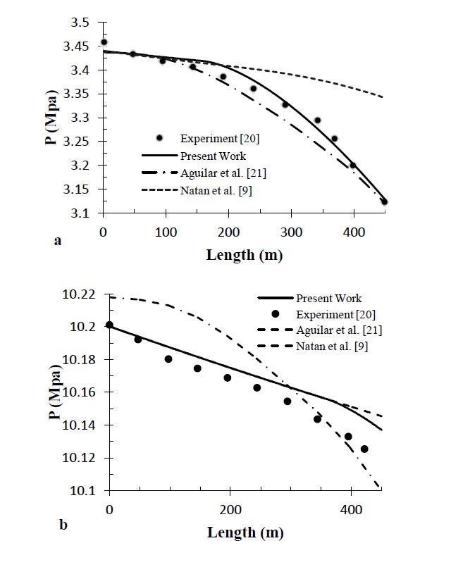
[9]	Natan S, Barnea D, Taitel Y (2003) Direct steam generation in parallel pipes. Int J Multiph Flow 29: 1669-1683. doi: 10.1016/j.ijmultiphaseflow.2003.07.002
[10]	Minzer U, Barnea D, Taitel Y (2006) Flow rate distribution in evaporating parallel pipes – modeling and experimental. Chem Eng Sci 61: 7249-7259. doi: 10.1016/j.ces.2006.08.026
[11]	Taitel Y, Barnea D (2011) Transient solution for flow of evaporating fluid in parallel pipes using analysis based on flow patterns. Int J Multiph Flow 37: 469-474. doi: 10.1016/j.ijmultiphaseflow.2011.01.002
[12]	Eck M, Steinmann WD (2005) Modelling and design of direct solar steam generating collector fields. J Sol Energy Eng 127: 371-380. doi: 10.1115/1.1849225
[13]	Friedel L, Modellgesetz fur den Reibungsdruckverlust in der Zweiphasenströmung. VDI-Forschungsheft 1975, 572.
[14]	Chisholm D (1980) Two-phase flow in bends. Int J Multiph Flow 6: 363-367. doi: 10.1016/0301-9322(80)90028-2
[15]	Bonilla J, Yebra LJ, Dormido S (2012) Chattering in dynamic mathematical two-phase flow models. Appl Math Model 36: 2067-2081.
[16]	Lobón DH, Valenzuela L (2013) Impact of pressure losses in small-sized parabolic-trough collectors for direct steam generation. Energy 61: 502-512. doi: 10.1016/j.energy.2013.08.049
[17]	Serrano-Aguilera JJ, Valenzuela L, Parras L (2014) Thermal 3D model for direct solar steam generation under superheated conditions. Appl Energy 132: 370-382. doi: 10.1016/j.apenergy.2014.07.035
[18]	Silva R, Pérez M, Berenguel M, et al. (2014) Uncertainty and global sensitivity analysis in the design of parabolic-trough direct steam generation plants for process heat applications. Appl Energy 121: 233-244. doi: 10.1016/j.apenergy.2014.01.095
[19]	Elsafi AM (2015) On thermo-hydraulic modeling of direct steam generation. Sol Energy 120: 636-650. doi: 10.1016/j.solener.2015.08.008
[20]	Zarza E, Valenzuela L, León J, et al. (2004) Direct Steam in parabolic troughs: Final results and conclusions of the DISS project. Energy 29: 635-644. doi: 10.1016/S0360-5442(03)00172-5
[21]	Aguilar-Gastelum F, Moya SL, Cazarez-Candia O, et al. (2014) Theoretical study of direct steam generation in two parallel pipes. Energy Procedia 57: 2265-2274. doi: 10.1016/j.egypro.2014.10.234
[22]	Odeh SD, Morrison GL, Behnia M (1998) Modelling of parabolic trough direct steam generation solar collectors. Solar Energy 62: 395-406. doi: 10.1016/S0038-092X(98)00031-0

This article has been cited by:

1.	Jia-Bao Liu, Saad Ihsan Butt, Jamshed Nasir, Adnan Aslam, Asfand Fahad, Jarunee Soontharanon, Jensen-Mercer variant of Hermite-Hadamard type inequalities via Atangana-Baleanu fractional operator, 2022, 7, 2473-6988, 2123, 10.3934/math.2022121
2.	Hasib Khan, Jehad Alzabut, Anwar Shah, Sina Etemad, Shahram Rezapour, Choonkil Park, A study on the fractal-fractional tobacco smoking model, 2022, 7, 2473-6988, 13887, 10.3934/math.2022767
3.	Hasib Khan, Muhammad Ibrahim, Abdel-Haleem Abdel-Aty, M. Motawi Khashan, Farhat Ali Khan, Aziz Khan, A fractional order Covid-19 epidemic model with Mittag-Leffler kernel, 2021, 148, 09600779, 111030, 10.1016/j.chaos.2021.111030
4.	Krunal B. Kachhia, Chaos in fractional order financial model with fractal–fractional derivatives, 2023, 7, 26668181, 100502, 10.1016/j.padiff.2023.100502
5.	Hari M. Srivastava, Khaled Mohammed Saad, Walid M. Hamanah, Certain New Models of the Multi-Space Fractal-Fractional Kuramoto-Sivashinsky and Korteweg-de Vries Equations, 2022, 10, 2227-7390, 1089, 10.3390/math10071089
6.	Hasnaa H Alzahrani, Marco Lucchesi, Kassem Mustapha, Olivier P Le Maître, Omar M Knio, Bayesian calibration of order and diffusivity parameters in a fractional diffusion equation, 2021, 5, 2399-6528, 085014, 10.1088/2399-6528/ac1507
7.	Jagdev Singh, Arpita Gupta, Dumitru Baleanu, On the analysis of an analytical approach for fractional Caudrey-Dodd-Gibbon equations, 2022, 61, 11100168, 5073, 10.1016/j.aej.2021.09.053
8.	Xiaojun Zhou, Yue Dai, A spectral collocation method for the coupled system of nonlinear fractional differential equations, 2022, 7, 2473-6988, 5670, 10.3934/math.2022314
9.	Nauman Ahmed, Ali Raza, Ali Akgül, Zafar Iqbal, Muhammad Rafiq, Muhammad Ozair Ahmad, Fahd Jarad, New applications related to hepatitis C model, 2022, 7, 2473-6988, 11362, 10.3934/math.2022634
10.	Esra Karatas Akgül, Wasim Jamshed, Kottakkaran Sooppy Nisar, S.K. Elagan, Nawal A. Alshehri, On solutions of gross domestic product model with different kernels, 2022, 61, 11100168, 1289, 10.1016/j.aej.2021.06.067
11.	Rubayyi T. Alqahtani, Shabir Ahmad, Ali Akgül, On Numerical Analysis of Bio-Ethanol Production Model with the Effect of Recycling and Death Rates under Fractal Fractional Operators with Three Different Kernels, 2022, 10, 2227-7390, 1102, 10.3390/math10071102
12.	A. DLAMINI, EMILE F. DOUNGMO GOUFO, M. KHUMALO, CHAOTIC BEHAVIOR OF MODIFIED STRETCH–TWIST–FOLD FLOW UNDER FRACTAL-FRACTIONAL DERIVATIVES, 2022, 30, 0218-348X, 10.1142/S0218348X22402071
13.	Anwar Zeb, Abdon Atangana, Zareen A. Khan, Salih Djillali, A robust study of a piecewise fractional order COVID-19 mathematical model, 2022, 61, 11100168, 5649, 10.1016/j.aej.2021.11.039
14.	Shabir Ahmad, Aman Ullah, Ali Akgül, Manuel De la Sen, A study of fractional order Ambartsumian equation involving exponential decay kernel, 2021, 6, 2473-6988, 9981, 10.3934/math.2021580
15.	Raheel Kamal, Gul Rahmat, Kamal Shah, Ricardo Escobar, On the Numerical Approximation of Three-Dimensional Time Fractional Convection-Diffusion Equations, 2021, 2021, 1563-5147, 1, 10.1155/2021/4640467
16.	Kaihong Zhao, Shuang Ma, Ulam-Hyers-Rassias stability for a class of nonlinear implicit Hadamard fractional integral boundary value problem with impulses, 2022, 7, 2473-6988, 3169, 10.3934/math.2022175
17.	Kamsing Nonlaopon, Muhammad Naeem, Ahmed M. Zidan, Rasool Shah, Ahmed Alsanad, Abdu Gumaei, Muhammad Imran Asjad, Numerical Investigation of the Time-Fractional Whitham–Broer–Kaup Equation Involving without Singular Kernel Operators, 2021, 2021, 1099-0526, 1, 10.1155/2021/7979365
18.	Saima Rashid, Rehana Ashraf, Ebenezer Bonyah, Azhar Hussain, On Analytical Solution of Time-Fractional Biological Population Model by means of Generalized Integral Transform with Their Uniqueness and Convergence Analysis, 2022, 2022, 2314-8888, 1, 10.1155/2022/7021288
19.	Khadija Tul Kubra, Rooh Ali, Modeling and analysis of novel COVID-19 outbreak under fractal-fractional derivative in Caputo sense with power-law: a case study of Pakistan, 2023, 2363-6203, 10.1007/s40808-023-01747-w
20.	ZAREEN A. KHAN, KAMAL SHAH, BAHAAELDIN ABDALLA, THABET ABDELJAWAD, A NUMERICAL STUDY OF COMPLEX DYNAMICS OF A CHEMOSTAT MODEL UNDER FRACTAL-FRACTIONAL DERIVATIVE, 2023, 31, 0218-348X, 10.1142/S0218348X23401813
21.	Kamal Shah, Thabet Abdeljawad, On complex fractal-fractional order mathematical modeling of CO 2 emanations from energy sector, 2024, 99, 0031-8949, 015226, 10.1088/1402-4896/ad1286
22.	Samy A. Abdelhafeez, Anas A. M. Arafa, Yousef H. Zahran, Ibrahim S. I. Osman, Moutaz Ramadan, Adapting Laplace residual power series approach to the Caudrey Dodd Gibbon equation, 2024, 14, 2045-2322, 10.1038/s41598-024-57780-x
23.	Krunal B. Kachhia, Prit P. Parmar, A novel fractional mask for image denoising based on fractal–fractional integral, 2024, 11, 26668181, 100833, 10.1016/j.padiff.2024.100833
24.	Harpreet Kaur, Amanpreet Kaur, Palwinder Singh, Scale-3 Haar wavelet-based method of fractal-fractional differential equations with power law kernel and exponential decay kernel, 2024, 13, 2192-8029, 10.1515/nleng-2022-0380
25.	Muhammad Farman, Changjin Xu, Perwasha Abbas, Aceng Sambas, Faisal Sultan, Kottakkaran Sooppy Nisar, Stability and chemical modeling of quantifying disparities in atmospheric analysis with sustainable fractal fractional approach, 2025, 142, 10075704, 108525, 10.1016/j.cnsns.2024.108525
26.	Ashish Rayal, System of fractal-fractional differential equations and Bernstein wavelets: a comprehensive study of environmental, epidemiological, and financial applications, 2025, 100, 0031-8949, 025236, 10.1088/1402-4896/ada592
27.	Mashael M. AlBaidani, Abdul Hamid Ganie, Adnan Khan, Fahad Aljuaydi, An Approximate Analytical View of Fractional Physical Models in the Frame of the Caputo Operator, 2025, 9, 2504-3110, 199, 10.3390/fractalfract9040199

Reader Comments

Your name:*

Email:*
© 2016 the Author(s), licensee AIMS Press. This is an open access article distributed under the terms of the Creative Commons Attribution License (http://creativecommons.org/licenses/by/4.0)