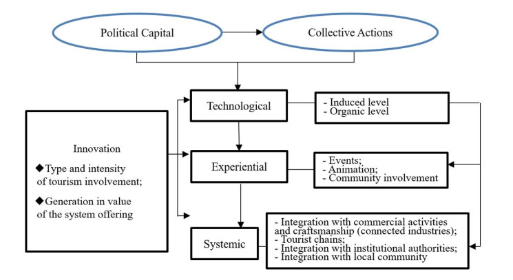
This study explores the service innovation model of Taiwan's Yingge Historical Street of Ceramics and analyzes how political capital and public-private partnerships (PPPs) influence service innovation development in the district. By adopting a case-study approach, data was collected from literature and secondary sources. Findings reveal three aspects of the service innovation model: (1) innovation based on cultural heritage, utilizing ceramic culture and technology to offer diverse cultural experiences; (2) community participation as the core, enhancing cohesion, identity, and promoting cultural heritage development; and (3) service innovation mechanism through PPPs, integrating public and private resources/capabilities to enhance efficiency and quality. The study highlights the significant impact of political capital (government support, funding, regulatory frameworks, and local groups' political influence) and PPPs (collective public-private actions including resource integration, cooperation norms, trust-building, and value co-creation) on service innovation. This contributes theoretically and practically to understanding service innovation mechanisms in cultural districts and promoting their development.
Citation: YiFu Hsu, ChunLiang Chen. Service innovation models in cultural districts: A case of Taiwan Yingge Historical Street[J]. Urban Resilience and Sustainability, 2024, 2(4): 371-389. doi: 10.3934/urs.2024020
This study explores the service innovation model of Taiwan's Yingge Historical Street of Ceramics and analyzes how political capital and public-private partnerships (PPPs) influence service innovation development in the district. By adopting a case-study approach, data was collected from literature and secondary sources. Findings reveal three aspects of the service innovation model: (1) innovation based on cultural heritage, utilizing ceramic culture and technology to offer diverse cultural experiences; (2) community participation as the core, enhancing cohesion, identity, and promoting cultural heritage development; and (3) service innovation mechanism through PPPs, integrating public and private resources/capabilities to enhance efficiency and quality. The study highlights the significant impact of political capital (government support, funding, regulatory frameworks, and local groups' political influence) and PPPs (collective public-private actions including resource integration, cooperation norms, trust-building, and value co-creation) on service innovation. This contributes theoretically and practically to understanding service innovation mechanisms in cultural districts and promoting their development.

| [1] |
Matarrita-Cascante D, Brennan MA, Luloff A (2010) Community agency and sustainable tourism development: The case of La Fortuna, Costa Rica. J Sustain Tour 18: 735–756. https://doi.org/10.1080/09669581003653526 doi: 10.1080/09669581003653526

|
| [2] | Evans G (2005) Measure for measure: Evaluating the evidence of culture's contribution to regeneration. Urban Stud 42: 959–983. Available from: http://www.jstor.org/stable/43197307. |
| [3] |
Lin CP, Chen SH, Trac LVT, et al. (2021) An expert-knowledge-based model for evaluating cultural tourism strategies: A case of Tainan City, Taiwan. J Hosp Tour Manag 49: 214–225. https://doi.org/10.1016/j.jhtm.2021.08.020 doi: 10.1016/j.jhtm.2021.08.020
|
| [4] |
Emery M, Flora C (2006) Spiraling-up: Mapping community transformation with community capitals framework. Community Dev 37: 19–35. https://doi.org/10.1080/15575330609490152 doi: 10.1080/15575330609490152
|
| [5] |
Della Corte V, Savastano I, Storlazzi A (2009) Service innovation in cultural heritages management and valorization. Int J Qual Serv Sci 1: 225–240. https://doi.org/10.1108/17566690911004177 doi: 10.1108/17566690911004177
|
| [6] |
Chen T, Park H, Rajwani T (2024) Diverse human resource slack and firm innovation: Evidence from politically connected firms. Int Bus Rev 33: 102244. https://doi.org/10.1016/j.ibusrev.2023.102244 doi: 10.1016/j.ibusrev.2023.102244
|
| [7] |
Berger AN, Karakaplan MU, Roman RA (2023) Whose bailout is it anyway? The roles of politics in PPP bailouts of small businesses vs. banks. J Financial Intermediation 56: 101044. https://doi.org/10.1016/j.jfi.2023.101044 doi: 10.1016/j.jfi.2023.101044
|
| [8] |
Hodge GA, Greve C (2007) Public–private partnerships: An international performance review. Public Adm Rev 67: 545–558. https://doi.org/10.1111/j.1540-6210.2007.00736.x doi: 10.1111/j.1540-6210.2007.00736.x
|
| [9] |
Osei-Kyei R, Chan APC (2015) Review of studies on the Critical Success Factors for Public–Private Partnership (PPP) projects from 1990 to 2013. Int J Project Manage 33: 1335–1346. https://doi.org/10.1016/j.ijproman.2015.02.008 doi: 10.1016/j.ijproman.2015.02.008
|
| [10] |
Ostrom E (1998) A behavioral approach to the rational choice theory of collective action: Presidential address, American Political Science Association, 1997. Am Polit Sci Rev 92: 1–22. https://doi.org/10.2307/2585925 doi: 10.2307/2585925
|
| [11] |
Kim H, Kim H, Woosnam KM (2023) Collaborative governance and conflict management in cultural heritage-led regeneration projects: The case of urban Korea. Habitat Int 134: 102767. https://doi.org/10.1016/j.habitatint.2023.102767 doi: 10.1016/j.habitatint.2023.102767
|
| [12] |
Kim H, Kim H, Woosnam KM (2023) Considering urban regeneration policy support: Perceived collaborative governance in cultural heritage-led regeneration projects of Korea. Habitat Int 140: 102921. https://doi.org/10.1016/j.habitatint.2023.102921 doi: 10.1016/j.habitatint.2023.102921
|
| [13] |
Li Z, Lin Y, Hooimeijer P, et al. (2024) Heritage conflict evolution: Changing framing strategies and opportunity structures in two heritage district redevelopment projects in China. Geoforum 149: 103959. https://doi.org/10.1016/j.geoforum.2024.103959 doi: 10.1016/j.geoforum.2024.103959
|
| [14] | Smith L (2006) Uses of Heritage, London: Routledge. https://doi.org/10.4324/9780203602263 |
| [15] | Casey KL (2005) Defining political capital: A reconsideration of Bourdieu's interconvertibility theory. |
| [16] | Cleere H (2012) Archaeological Heritage Management in the Modern World, London: Routledge. https://doi.org/10.4324/9780203060223 |
| [17] | Pine BJ, Gilmore JH (2011) The Experience Economy, Boston: Harvard Business Press. |
| [18] |
Chen CL (2022) Strategic sustainable service design for creative-cultural hotels: A multi-level and multi-domain view. Local Environ 27: 46–79. https://doi.org/10.1080/13549839.2021.2001796 doi: 10.1080/13549839.2021.2001796
|
| [19] |
Chen CL (2021) Cultural product innovation strategies adopted by the performing arts industry. Rev Manag Sci 15: 1139–1171. https://doi.org/10.1007/s11846-020-00393-1 doi: 10.1007/s11846-020-00393-1
|
| [20] |
Chen JS, Kerr D, Chou CY, et al. (2017) Business co-creation for service innovation in the hospitality and tourism industry. Int J Contemp Hosp Manag 29: 1522–1540. https://doi.org/10.1108/IJCHM-06-2015-0308 doi: 10.1108/IJCHM-06-2015-0308
|
| [21] |
Hincapié M, Díaz C, Zapata-Cárdenas MI, et al. (2021) Augmented reality mobile apps for cultural heritage reactivation. Comput Electr Eng 93: 107281. https://doi.org/10.1016/j.compeleceng.2021.107281 doi: 10.1016/j.compeleceng.2021.107281
|
| [22] |
Lyu Y, Abd Malek MI, Jaafar NH, et al. (2023) Unveiling the potential of space syntax approach for revitalizing historic urban areas: A case study of Yushan Historic District, China. Front Archit Res 12: 1144–1156. https://doi.org/10.1016/j.foar.2023.08.004 doi: 10.1016/j.foar.2023.08.004
|
| [23] |
Vargo SL, Lusch RF (2017) Service-dominant logic 2025. Int J Res Mark 34: 46–67. https://doi.org/10.1016/j.ijresmar.2016.11.001 doi: 10.1016/j.ijresmar.2016.11.001
|
| [24] |
Aal K, Di Pietro L, Edvardsson B, et al. (2016) Innovation in service ecosystems. J Serv Manag 27: 619–651. https://doi.org/10.1108/JOSM-02-2015-0044 doi: 10.1108/JOSM-02-2015-0044
|
| [25] |
Vargo SL, Lusch RF (2008) Service-dominant logic: Continuing the evolution. J Acad Mark Sci 36: 1–10. https://doi.org/10.1007/s11747-007-0069-6 doi: 10.1007/s11747-007-0069-6
|
| [26] |
Hörger C, Ward P (2023) Coordination mechanisms and the role of taskscape in value co-creation: The British 'milkman'. J Bus Res 162: 113849. https://doi.org/10.1016/j.jbusres.2023.113849 doi: 10.1016/j.jbusres.2023.113849
|
| [27] |
Vargo SL (2020) From promise to perspective: Reconsidering value propositions from a service-dominant logic orientation. Ind Mark Manag 87: 309–311. https://doi.org/10.1016/j.indmarman.2019.10.013 doi: 10.1016/j.indmarman.2019.10.013
|
| [28] |
Bennett N, Lemelin RH, Koster R, et al. (2012) A capital assets framework for appraising and building capacity for tourism development in aboriginal protected area gateway communities. Tour Manag 33: 752–766. https://doi.org/https://doi.org/10.1016/j.tourman.2011.08.009 doi: 10.1016/j.tourman.2011.08.009
|
| [29] |
Flora CB, Flora JL (1993) Entrepreneurial social infrastructure: A necessary ingredient. Ann Am Acad Polit Soc Sci 529: 48–58. https://doi.org/10.1177/000271629352900100 doi: 10.1177/000271629352900100
|
| [30] |
Hale J, Irish A, Carolan M, et al. (2023) A systematic review of cultural capital in US community development research. J Rural Stud 103: 103113. https://doi.org/10.1016/j.jrurstud.2023.103113 doi: 10.1016/j.jrurstud.2023.103113
|
| [31] | Flora CB (2016) Rural Communities: Legacy+ Change, New York: Routledge. https://doi.org/10.4324/9780429494697 |
| [32] | Green GP, Haines A (2016) Asset Building & Community Development, Sage publications. https://doi.org/10.4135/9781483398631 |
| [33] |
Turner RS (1999) Entrepreneurial neighborhood initiatives: Political capital in community development. Econ Dev Q 13: 15–22. https://doi.org/10.1177/089124249901300103 doi: 10.1177/089124249901300103
|
| [34] |
McDonald C, Kirk-Brown A, Frost L, et al. (2013) Partnerships and integrated responses to rural decline: The role of collective efficacy and political capital in Northwest Tasmania, Australia. J Rural Stud 32: 346–356. https://doi.org/10.1016/j.jrurstud.2013.08.003 doi: 10.1016/j.jrurstud.2013.08.003
|
| [35] |
Núñez APB, Gutiérrez-Montes I, Hernández-Núñez HE, et al. (2023) Diverse farmer livelihoods increase resilience to climate variability in southern Colombia. Land Use Policy 131: 106731. https://doi.org/10.1016/j.landusepol.2023.106731 doi: 10.1016/j.landusepol.2023.106731
|
| [36] |
Elsahn ZF, Benson-Rea M (2018) Political schemas and corporate political activities during foreign market entry: A micro-process perspective. Manag Int Rev 58: 771–811. https://doi.org/10.1007/s11575-018-0350-6 doi: 10.1007/s11575-018-0350-6
|
| [37] |
Xia T, Liu X (2022) The innovation paradox of TMT political capital in transition economy firms. J Bus Res 142: 775–790. https://doi.org/10.1016/j.jbusres.2022.01.011 doi: 10.1016/j.jbusres.2022.01.011
|
| [38] |
Aquino RS, Lück M, Schänzel HA (2018) A conceptual framework of tourism social entrepreneurship for sustainable community development. J Hosp Tour Manag 37: 23–32. https://doi.org/https://doi.org/10.1016/j.jhtm.2018.09.001 doi: 10.1016/j.jhtm.2018.09.001
|
| [39] |
Pigg K, Gasteyer S, Martin K, et al. (2013) The community capitals framework: An empirical examination of internal relationships. Community Dev 44: 492–502. http://dx.doi.org/10.1080/15575330.2013.814698 doi: 10.1080/15575330.2013.814698
|
| [40] |
Sørensen JFL, Svendsen GLH (2023) What makes peripheral places matter? Applying the concept of political capital within a multiple capital framework. J Rural Stud 103: 103136. https://doi.org/10.1016/j.jrurstud.2023.103136 doi: 10.1016/j.jrurstud.2023.103136
|
| [41] |
Zekeri AA (2013) Community capital and local economic development efforts. Prof Agric Workers J 1. http://dx.doi.org/10.22004/ag.econ.236728 doi: 10.22004/ag.econ.236728
|
| [42] |
Jung TH, Lee J, Yap MH, et al. (2015) The role of stakeholder collaboration in culture-led urban regeneration: A case study of the Gwangju project, Korea. Cities 44: 29–39. https://doi.org/10.1016/j.cities.2014.12.003 doi: 10.1016/j.cities.2014.12.003
|
| [43] |
Montalto V, Alberti V, Panella F, et al. (2023) Are cultural cities always creative? An empirical analysis of culture-led development in 190 European cities. Habitat Int 132: 102739. https://doi.org/10.1016/j.habitatint.2022.102739 doi: 10.1016/j.habitatint.2022.102739
|
| [44] | Carroll P, Steane P (2000) Public-private partnerships: Sectoral perspectives, In: Public-Private Partnerships, Routledge, 54–74. |
| [45] |
Azarian M, Shiferaw AT, Lædre O, et al. (2023) Project ownership in public-private partnership (PPP) projects of Norway. Procedia Comput Sci 219: 1838–1846. https://doi.org/10.1016/j.procs.2023.01.481 doi: 10.1016/j.procs.2023.01.481
|
| [46] |
Brown TL, Potoski M, Van Slyke DM (2006) Managing public service contracts: Aligning values, institutions, and markets. Public Adm Rev 66: 323–331. https://doi.org/https://doi.org/10.1111/j.1540-6210.2006.00590.x00 doi: 10.1111/j.1540-6210.2006.00590.x00
|
| [47] |
Zhao Y (2015) 'China's leading historical and cultural city': Branding Dali City through public–private partnerships in Bai architecture revitalization. Cities 49: 106–112. https://doi.org/10.1016/j.cities.2015.07.009 doi: 10.1016/j.cities.2015.07.009
|
| [48] |
Rufin C, Rivera-Santos M (2012) Between commonweal and competition: Understanding the governance of public–private partnerships. J Manag 38: 1634–1654. https://doi.org/10.1177/0149206310373948 doi: 10.1177/0149206310373948
|
| [49] | Stephen O (2000) Public-Private Partnerships: Theory and Practice in International Perspective. London: Routledge. https://doi.org/10.4324/9780203207116 |
| [50] |
Robaczewska J, Vanhaverbeke W, Lorenz A (2019) Applying open innovation strategies in the context of a regional innovation ecosystem: The case of Janssen Pharmaceuticals. Glob Transit 1: 120–131. https://doi.org/10.1016/j.glt.2019.05.001 doi: 10.1016/j.glt.2019.05.001
|
| [51] |
Absalyamov T (2015) Tatarstan model of public-private partnership in the field of cultural heritage preservation. Procedia: Soc Behav Sci 188: 214–217. https://doi.org/10.1016/j.sbspro.2015.03.375 doi: 10.1016/j.sbspro.2015.03.375
|
| [52] |
Rossetti G, Quinn B (2021) Understanding the cultural potential of rural festivals: A conceptual framework of cultural capital development. J Rural Stud 86: 46–53. https://doi.org/10.1016/j.jrurstud.2021.05.009 doi: 10.1016/j.jrurstud.2021.05.009
|
| [53] | Yin RK (2009) Case Study Research: Design and Methods, Sage Publications. |
| [54] | Stake RE (1995) Case Study Research, Thousand Oaks, CA: Sage Publications. |
| [55] | Patton MQ (2014) Qualitative Research & Evaluation Methods: Integrating Theory and Practice: Thousand Oaks, CA: SAGE Publications. |
| [56] | Denzin NK (2017) The Research Act: A Theoretical Introduction to Sociological Methods, New York: Routledge. https://doi.org/10.4324/9781315134543 |
| [57] |
Lin CL (2019) Establishing environment sustentation strategies for urban and rural/town tourism based on a hybrid MCDM approach. Curr Issues Tour 23: 2360–2395. https://doi.org/10.1080/13683500.2019.1642308 doi: 10.1080/13683500.2019.1642308
|
| [58] |
Berry LL, Zeithaml VA, Parasuraman A (1985) Quality counts in services, too. Bus Horiz 28: 44–52. https://doi.org/10.1016/0007-6813(85)90008-4 doi: 10.1016/0007-6813(85)90008-4
|
| [59] |
Nishant R, Kennedy M, Corbett J (2020) Artificial intelligence for sustainability: Challenges, opportunities, and a research agenda. Int J Inf Manage 53: 102104. https://doi.org/10.1016/j.ijinfomgt.2020.102104 doi: 10.1016/j.ijinfomgt.2020.102104
|
Figures(1)
YiFu Hsu, ChunLiang Chen. Service innovation models in cultural districts: A case of Taiwan Yingge Historical Street[J]. Urban Resilience and Sustainability, 2024, 2(4): 371-389. doi: 10.3934/urs.2024020


 DownLoad: