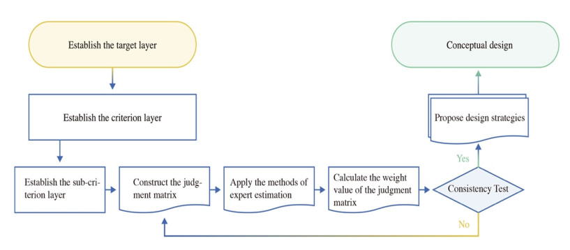
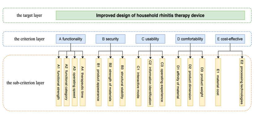
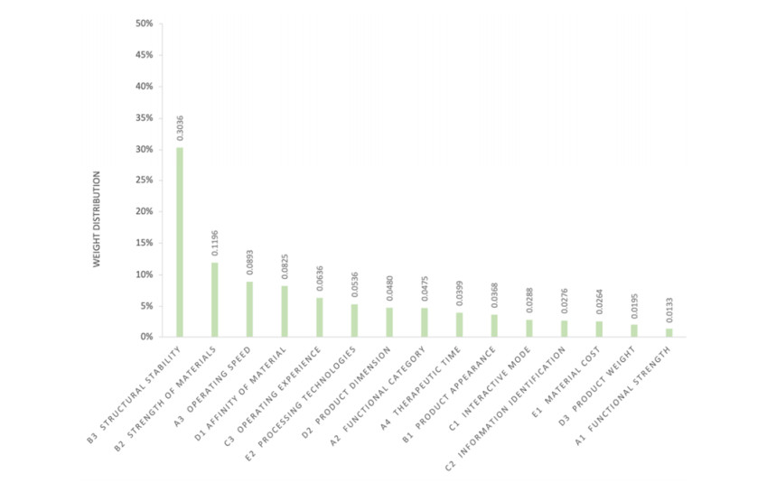
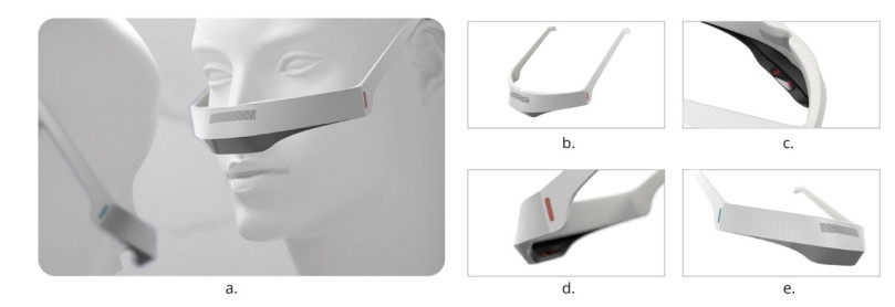
To improve the scientificity of household medical product design for rhinitis patients, this study used the analytic hierarchy process (AHP) to provide guidance for household medical product design strategy. In the process of design decision-making, the identification of user needs and the evaluation of the scheme depend heavily on the designer's experience and knowledge. The main contribution of this paper is to evaluate the design elements through the AHP method and apply it to the actual design work. This work can greatly reduce the risk in design decisions. First, the AHP model and evaluation matrix of design elements were established and sorted out by semantic analysis of users' research results. Second, an expert group was invited to score using the 1–9 scale method. Then, the geometric mean method was used to calculate the weight shares of different indicators so as to rank them. Finally, the strategy was proposed based on ranking indicator weights, and product design was carried out. The application of AHP can make the product design process more objective and rigorous. The design scheme of this study can provide references and ideas to promote the vigorous development of household medical products for rhinitis patients.
Citation: Wei Liu, Yi Huang, Yue Sun, Changlong Yu. Research on design elements of household medical products for rhinitis based on AHP[J]. Mathematical Biosciences and Engineering, 2023, 20(5): 9003-9017. doi: 10.3934/mbe.2023395
To improve the scientificity of household medical product design for rhinitis patients, this study used the analytic hierarchy process (AHP) to provide guidance for household medical product design strategy. In the process of design decision-making, the identification of user needs and the evaluation of the scheme depend heavily on the designer's experience and knowledge. The main contribution of this paper is to evaluate the design elements through the AHP method and apply it to the actual design work. This work can greatly reduce the risk in design decisions. First, the AHP model and evaluation matrix of design elements were established and sorted out by semantic analysis of users' research results. Second, an expert group was invited to score using the 1–9 scale method. Then, the geometric mean method was used to calculate the weight shares of different indicators so as to rank them. Finally, the strategy was proposed based on ranking indicator weights, and product design was carried out. The application of AHP can make the product design process more objective and rigorous. The design scheme of this study can provide references and ideas to promote the vigorous development of household medical products for rhinitis patients.

| [1] |
Z. Zheng, Y. Y. Yu, A review of recent advances in exosomes and allergic rhinitis, Front. Pharmacol., 13 (2022), 1096984. https://doi.org/10.3389/fphar.2022.1096984 doi: 10.3389/fphar.2022.1096984

|
| [2] |
L. Cheng, Revising allergic rhinitis guidelines to standardize clinical diagnosis and treatment, Chin. J. Otorhinolaryngol. Head Neck Surg., 57 (2022), 413–417. https://doi.org/10.3760/cma.j.cn115330-20220325-00134 doi: 10.3760/cma.j.cn115330-20220325-00134
|
| [3] |
Y. Shen, E. M. Nasab, F. Hassanpour, S. S. Athari, The effects of combined therapeutic protocol on allergic rhinitis symptoms and molecular determinants, Iran. J. Allergy Asthma Immunol., 21 (2022), 141–150. https://doi.org/10.18502/ijaai.v21i2.9222 doi: 10.18502/ijaai.v21i2.9222
|
| [4] |
Z. Wu, H. R. Karimi, C. Dang, An approximation algorithm for graph partitioning via deterministic annealing neural network, Neural Networks, 117 (2019), 191–200. https://doi.org/10.1016/j.neunet.2019.05.010 doi: 10.1016/j.neunet.2019.05.010
|
| [5] |
T. C. Wang, T. H. Chang, Application of TOPSIS in evaluating initial training aircraft under a fuzzy environment, Expert Syst. Appl., 33 (2007), 870–880. https://doi.org/10.1016/j.eswa.2006.07.003 doi: 10.1016/j.eswa.2006.07.003
|
| [6] |
J. Zhou, C. Lei, Q. Zheng, G. J. Ding, X. C. Bian, Development of hydropower construction management system integrating grey theory and quality function deployment, J. Yangtze River Sci. Res. Inst., 36 (2019), 151. https://doi.org/10.11988/ckyyb.20180700 doi: 10.11988/ckyyb.20180700
|
| [7] |
K. Fröhlingsdorf, M. Dreßen, S. Pischinger, C. Steffens, S. Heuer, Analysis of the influence of Image Processing, Feature Selection, and Decision Tree Classification on noise separation of electric vehicle powertrains, SAE Int. J. Veh. Dyn. Stab. NVH, 7 (2022), 23–33. https://doi.org/10.4271/10-07-01-0002 doi: 10.4271/10-07-01-0002
|
| [8] |
Y. Xiu, X. Wang, H. Li, W. Lu, V. Nguyen, J. Jiang, et al., Comparative vibration isolation assessment of two seat suspension models with different negative stiffness structure, SAE Int. J. Veh. Dyn. Stab. NVH, 7 (2022), 99–112. https://doi.org/10.4271/10-07-01-0007 doi: 10.4271/10-07-01-0007
|
| [9] |
X. Wang, A. L. Osvalder, P. Höstmad, Influence of sound and vibration on perceived overall ride comfort—A comparison between an electric vehicle and a combustion engine vehicle, SAE Int. J. Veh. Dyn. Stab. NVH, 7 (2023). https://doi.org/10.4271/10-07-02-0010 doi: 10.4271/10-07-02-0010
|
| [10] |
M. Irfan, R. M. Elavarasan, M. Ahmad, M. Mohsin, V. Dagar, Y. Hao, Prioritizing and overcoming biomass energy barriers: Application of AHP and G-TOPSIS approaches, Technol. Forecasting Social Change, 177 (2022), 121524. https://doi.org/10.1016/j.techfore.2022.121524 doi: 10.1016/j.techfore.2022.121524
|
| [11] | F. E. Vladimirovna, K. A. Georgievna, Comprehensive approach to identifying ent diseases that could lead to a hearing pathology in children, Pract. Oriented Sci. UAE–RUSSIA–INDIA, 2022 (2022). https://doi.org/10.34660/INF.2022.20.37.185 |
| [12] |
J. Cook, A. McCombe, A. Jones, Laser treatment of rhinitis—1 year follow up, Clin. Otolaryngol. Allied Sci., 18 (1993), 209–211. https://doi.org/10.1111/j.1365-2273.1993.tb00832.x doi: 10.1111/j.1365-2273.1993.tb00832.x
|
| [13] |
C. Zhou, X. Luo, T. Huang, T. Zhou, Function matching of terminal modules of intelligent furniture for elderly based on wireless sensor network, IEEE Access, 8 (2020), 132481–132488. https://doi.org/10.1109/ACCESS.2020.3009732 doi: 10.1109/ACCESS.2020.3009732
|
| [14] |
D. van Eijk, J. van Kuijk, F. Hoolhorst, C. Kim, C. Harkema, S. Dorrestijn, Design for usability: Practice-oriented research for User-centered product design, Work, 41 (2012), 1008–1015. https://doi.org/10.3233/WOR-2012-1010-1008 doi: 10.3233/WOR-2012-1010-1008
|
| [15] |
R. W. Saaty, The analytic hierarchy process—what it is and how it is used, Math. Modell., 9 (1987), 161–176. https://doi.org/10.1016/0270-0255(87)90473-8 doi: 10.1016/0270-0255(87)90473-8
|
| [16] |
L. T. Xia, C. H. Ho, X. M. Lin, Evaluation of the elderly health examination app based on the comprehensive evaluation method of AHP-fuzzy theory, Math. Biosci. Eng., 18 (2021), 4731–4742. https://doi.org/10.3934/mbe.2021240 doi: 10.3934/mbe.2021240
|
| [17] |
Y. Moustafa, H. G. E. Nady, M. M. Saber, O. A. Dabbous, T. B. Kamel, K. G. Abel-Wahhab, et al., Assessment of allergic rhinitis among children after low-level laser therapy, Open Access Maced. J. Med. Sci., 7 (2019), 1968. https://doi.org/10.3889/oamjms.2019.477 doi: 10.3889/oamjms.2019.477
|
| [18] |
M. J. Fisher, E. Johansen, Human-centered design for medical devices and diagnostics in global health, Global Health Innovation, 3 (2020). https://doi.org/10.15641/ghi.v3i1.762 doi: 10.15641/ghi.v3i1.762
|
| [19] |
L. G. Vargas, An overview of the analytic hierarchy process and its applications, Eur. J. Oper. Res., 48 (1990), 2–8. https://doi.org/10.1016/0377-2217(90)90056-H doi: 10.1016/0377-2217(90)90056-H
|
| [20] |
C. X. Briceño-León, D. S. Sanchez-Ferrer, P. L. Iglesias-Rey, F. J. Martinez-Solano, D. Mora-Melia, Methodology for pumping station design based on analytic hierarchy process (AHP), Water, 13 (2021), 2886. https://doi.org/10.3390/w13202886 doi: 10.3390/w13202886
|
| [21] |
T. L. Zhu, Y. J. Li, C. J. Wu, H. Yue, Y. Q. Zhao, Research on the design of surgical auxiliary equipment based on AHP, QFD, and PUGH decision matrix, Math. Probl. Eng., 2022 (2022), 1–13. https://doi.org/10.1155/2022/4327390 doi: 10.1155/2022/4327390
|
| [22] |
H. Wang, Z. Sun, Research on multi decision making security performance of IoT identity resolution server based on AHP, Math. Biosci. Eng., 18 (2021), 3977–3992. https://doi.org/10.3934/mbe.2021199 doi: 10.3934/mbe.2021199
|
| [23] |
J. Franek, A. Kresta, Judgment scales and consistency measure in AHP, Procedia Econ. Finance, 12 (2014), 164–173. https://doi.org/10.1016/S2212-5671(14)00332-3 doi: 10.1016/S2212-5671(14)00332-3
|
| [24] |
W. Zhang, T. Lai, Y. Li, Risk assessment of water supply network operation based on ANP-Fuzzy comprehensive evaluation method, J. Pipeline Syst. Eng. Pract., 13 (2022), 4021068. https://doi.org/10.1061/(ASCE)PS.1949-1204.0000602 doi: 10.1061/(ASCE)PS.1949-1204.0000602
|
| [25] |
X. Li, L. Shen, R. Califano, The comparative study of thermal comfort and sleep quality for innovative designed mattress in hot weather, Sci. Technol. Built Environ., 26 (2020), 643–657. https://doi.org/10.1080/23744731.2020.1720445 doi: 10.1080/23744731.2020.1720445
|
| [26] |
L. Jiang, V. Cheung, S. Westland, P. A. Rhodes, L. Shen, L. Xu, The impact of color preference on adolescent children's choice of furniture, Color Res. Appl., 45 (2020), 754–767. https://doi.org/10.1002/col.22507 doi: 10.1002/col.22507
|
| [27] |
N. Yu, L. Hong, J. Guo, Analysis of upper-limb muscle fatigue in the process of rotary handling, Int. J. Ind. Ergon., 83 (2021), 103109. https://doi.org/10.1016/j.ergon.2021.103109 doi: 10.1016/j.ergon.2021.103109
|
| [28] | M. F. Ashby, K. Johnson, Materials and Design: the Art and Science of Material Selection in Product Design, Butterworth-Heinemann, 2013. |
| [29] |
L. W. Kuo, T. Chang, C. C. Lai, Research on product design modeling image and color psychological test, Displays, 71 (2022), 102108. https://doi.org/10.1016/j.displa.2021.102108 doi: 10.1016/j.displa.2021.102108
|
| [30] |
T. Huang, C. Zhou, X. Luo, J. Kaner, Study of ageing in complex interface interaction tasks: based on combined eye-movement and HRV bioinformatic feedback, Int. J. Environ. Res. Public Health, 19 (2022), 16937. https://doi.org/10.3390/ijerph192416937 doi: 10.3390/ijerph192416937
|
| [31] |
N. Yu, Z. Ouyang, H. Wang, D. Tao, L. Jing, The effects of smart home interface touch button design features on performance among young and senior users, Int. J. Environ. Res. Public Health, 19 (2022), 2391. https://doi.org/10.3390/ijerph19042391 doi: 10.3390/ijerph19042391
|
| [32] |
N. Yu, Z. Ouyang, H. Wang, Study on smart home interface design characteristics considering the influence of age difference: Focusing on sliders, Front. Psychol., 2022 (2022), 901. https://doi.org/10.3389/fpsyg.2022.828545 doi: 10.3389/fpsyg.2022.828545
|
| [33] |
J. J. Fang, L. M. Shen, Analysis of sagittal spinal alignment at the adolescent age: for furniture design, Ergonomics, 2022 (2022), 1–17. https://doi.org/10.1080/00140139.2022.2152491 doi: 10.1080/00140139.2022.2152491
|
| [34] |
Y. Chao, L. M. Shen, M. P. Liu, Mechanical characteristic and analytical model of novel air spring for ergonomic mattress, Mech. Ind., 22 (2021), 37. https://doi.org/10.1051/meca/2021035 doi: 10.1051/meca/2021035
|
| [35] |
H. Wang, D. Tao, N. Yu, X. Qu, Understanding consumer acceptance of healthcare wearable devices: An integrated model of UTAUT and TTF, Int. J. Med. Inf., 139 (2020), 104156. https://doi.org/10.1016/j.ijmedinf.2020.104156 doi: 10.1016/j.ijmedinf.2020.104156
|
Figures(4) / Tables(12)

Wei Liu, Yi Huang, Yue Sun, Changlong Yu. Research on design elements of household medical products for rhinitis based on AHP[J]. Mathematical Biosciences and Engineering, 2023, 20(5): 9003-9017. doi: 10.3934/mbe.2023395


 DownLoad: