Extracted features of national and continental daily biweekly growth rates of confirmed COVID-19 cases and deaths via Fourier analysis

Ray-Ming Chen; Ray-Ming Chen

doi:10.3934/mbe.2021311

Mathematical Biosciences and Engineering

2021, Volume 18, Issue 5: 6216-6238. doi: 10.3934/mbe.2021311

Previous Article Next Article

Research article Special Issues

Extracted features of national and continental daily biweekly growth rates of confirmed COVID-19 cases and deaths via Fourier analysis

Ray-Ming Chen ^,

Department of Mathematics and Statistics, Baise University, 21 Zhongshan No. 2 Road, Basie 533000, China

Academic Editor: Xiangtao Li

Received: 17 May 2021 Accepted: 13 July 2021 Published: 19 July 2021

Aims
By associating features with orthonormal bases, we analyse the values of the extracted features for the daily biweekly growth rates of COVID-19 confirmed cases and deaths on national and continental levels.

Methods
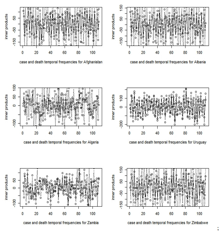
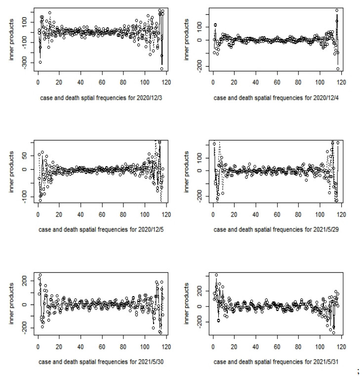
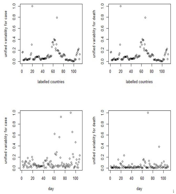
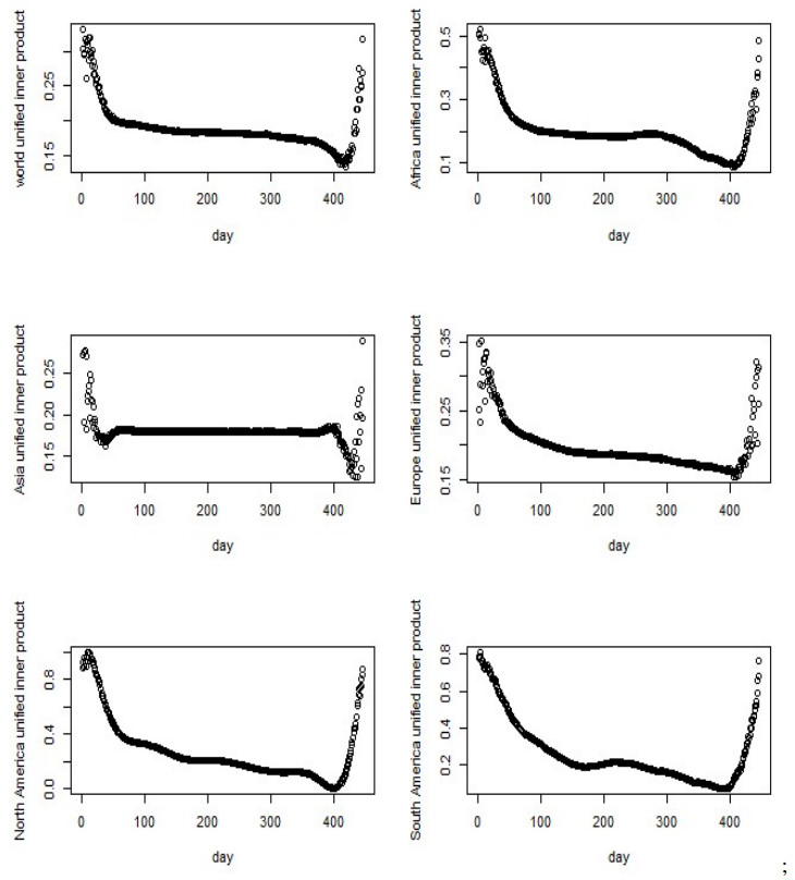
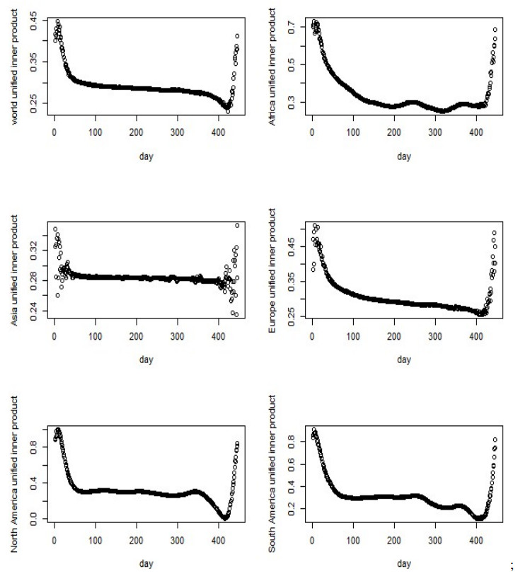
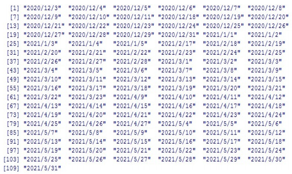
By adopting the concept of Fourier coefficients, we analyse the inner products with respect to temporal and spatial frequencies on national and continental levels. The input data are the global time series data with 117 countries over 109 days on a national level; and 6 continents over 447 days on a continental level. Next, we calculate the Euclidean distance matrices and their average variabilities, which measure the average discrepancy between one feature vector and all others. Then we analyse the temporal and spatial variabilities on a national level. By calculating the temporal inner products on a continental level, we derive and analyse the similarities between the continents.

Results
On the national level, the daily biweekly growth rates bear higher similarities in the time dimension than the ones in the space dimension. Furthermore, there exists a strong concurrency between the features for biweekly growth rates of cases and deaths. As far as the trends of the features are concerned, the features are stabler on the continental level, and less predictive on the national level. In addition, there are very high similarities between all the continents, except Asia.

Conclusions
The features for daily biweekly growth rates of cases and deaths are extracted via orthonormal frequencies. By tracking the inner products for the input data and the orthonormal features, we could decompose the evolutionary results of COVID-19 into some fundamental frequencies. Though the frequency-based techniques are applied, the interpretation of the features should resort to other methods. By analysing the spectrum of the frequencies, we reveal hidden patterns of the COVID-19 pandemic. This would provide some preliminary research merits for further insightful investigations. It could also be used to predict future trends of daily biweekly growth rates of COVID-19 cases and deaths.
- COVID-19,
- biweekly growth rates,
- variability,
- Fourier analysis,
- temporal and spatial
Citation: Ray-Ming Chen. Extracted features of national and continental daily biweekly growth rates of confirmed COVID-19 cases and deaths via Fourier analysis[J]. Mathematical Biosciences and Engineering, 2021, 18(5): 6216-6238. doi: 10.3934/mbe.2021311

Related Papers:

Abstract

Aims

By associating features with orthonormal bases, we analyse the values of the extracted features for the daily biweekly growth rates of COVID-19 confirmed cases and deaths on national and continental levels.

Methods

By adopting the concept of Fourier coefficients, we analyse the inner products with respect to temporal and spatial frequencies on national and continental levels. The input data are the global time series data with 117 countries over 109 days on a national level; and 6 continents over 447 days on a continental level. Next, we calculate the Euclidean distance matrices and their average variabilities, which measure the average discrepancy between one feature vector and all others. Then we analyse the temporal and spatial variabilities on a national level. By calculating the temporal inner products on a continental level, we derive and analyse the similarities between the continents.

Results

On the national level, the daily biweekly growth rates bear higher similarities in the time dimension than the ones in the space dimension. Furthermore, there exists a strong concurrency between the features for biweekly growth rates of cases and deaths. As far as the trends of the features are concerned, the features are stabler on the continental level, and less predictive on the national level. In addition, there are very high similarities between all the continents, except Asia.

Conclusions

The features for daily biweekly growth rates of cases and deaths are extracted via orthonormal frequencies. By tracking the inner products for the input data and the orthonormal features, we could decompose the evolutionary results of COVID-19 into some fundamental frequencies. Though the frequency-based techniques are applied, the interpretation of the features should resort to other methods. By analysing the spectrum of the frequencies, we reveal hidden patterns of the COVID-19 pandemic. This would provide some preliminary research merits for further insightful investigations. It could also be used to predict future trends of daily biweekly growth rates of COVID-19 cases and deaths.

References

[1]	Y. Wu, C. Chen, Y. Chan, The outbreak of COVID-19: An overview, J. Chin. Med. Assoc., 83 (2020), 217–220. doi: 10.1097/JCMA.0000000000000270
[2]	C. Huang, Y. Wang, X. Li, L. Ren, J. Zhao, Y. Hu, et al., Clinical features of patients infected with 2019 novel coronavirus in Wuhan, China, Lancet, 395 (2020), 497–506. doi: 10.1016/S0140-6736(20)30183-5
[3]	N. Davies, S. Abbott, R. Barnard, C. Jarvis, A. Kucharski, J. Munday, et al., Estimated transmissibility and impact of SARS-CoV-2 lineage B.1.1.7 in England, Science, 372 (2021), 497–506.
[4]	S. Madhi, V. Baillie, C. Cutland, M. Voysey, A. Koen, L. Fairlie, et al., Efficacy of the ChAdOx1 nCoV-19 Covid-19 Vaccine against the B.1.351 Variant, N. Engl. J. Med., 384 (2021), 1885–1898. doi: 10.1056/NEJMoa2102214
[5]	T. Tada, H. Zhou, B. Dcosta, M. Samanovic, M. Mulligan, N. Landau, The Spike Proteins of SARS-CoV-2 B.1.617 and B.1.618 Variants Identified in India Provide Partial Resistance to Vaccine-elicited and Therapeutic Monoclonal Antibodies, bioRxiv, 2021.
[6]	H. Tegally, E. Wilkinson, M. Giovanetti, A. Iranzadeh, V. Fonseca, J. Giandhari, et al., Detection of a SARS-CoV-2 variant of concern in South Africa, Nature, 592 (2001), 438–443.
[7]	R. Chen, Randomness for Nucleotide Sequences of SARS-CoV-2 and Its Related Subfamilies, Comput. Math. Methods Med., 2020 (2020), 1–8.
[8]	R. Chen, Distance matrices for nitrogenous bases and amino acids of SARS-CoV-2 via structural metric, J. Bioinf. Comput. Biol., 2021 (2021), 2150011.
[9]	C. Courtemanche, J. Garuccio, A. Le, J. Pinkston, A. Yelowitz, Strong Social Distancing Measures In The United States Reduced The COVID-19 Growth Rate: Study evaluates the impact of social distancing measures on the growth rate of confirmed COVID-19 cases across the United States, Health Aff., 39 (2020), 1237–1246. doi: 10.1377/hlthaff.2020.00608
[10]	R. Chen, On COVID-19 country containment metrics: a new approach, J. Decis. Syst., 2021 (2021), 1–18.
[11]	R. Chen. Track the dynamical features for mutant variants of COVID-19 in the UK, Math. Biosci. Eng., 18 (2021), 4572–4585.
[12]	J. Nick, M. Max, R. Peter, COVID-19 second wave mortality in Europe and the United States, Chaos, 31 (2021), 031105. doi: 10.1063/5.0041569
[13]	M. Cesar, B. Eduardo, S. Rafael, M. Carlos, B. Marcus, Strong correlations between power-law growth of COVID-19 in four continents and the inefficiency of soft quarantine strategies, Chaos, 30 (2020), 041102. doi: 10.1063/5.0009454
[14]	R. Omori, K. Mizumoto, G. Chowell, Changes in testing rates could mask the novel coronavirus disease (COVID-19) growth rate, Int. J. Infect. Dis., 94 (2020), 116-118. doi: 10.1016/j.ijid.2020.04.021
[15]	J. Machado, A. Lopes, Rare and extreme events: the case of COVID-19 pandemic, Nonlinear Dyn., 100 (2020), 2953–2972. doi: 10.1007/s11071-020-05680-w
[16]	J. Nick, M. Max, Trends in COVID-19 prevalence and mortality: A year in review, Phys. D, 425 (2021), 132968. doi: 10.1016/j.physd.2021.132968
[17]	J. Stübinger, L. Schneider, Epidemiology of coronavirus COVID-19: Forecasting the future incidence in different countries, in Healthcare, Multidisciplinary Digital Publishing Institute, 8 (2020), 99.
[18]	Z. Vasilios, P. G. Stavros, G. Zoe, Z. Efthimios, Clustering analysis of countries using the COVID-19 cases dataset, Data Brief, 31 (2020), 105787. doi: 10.1016/j.dib.2020.105787
[19]	R. Chen, Whether Economic Freedom Is Significantly Related to Death of COVID-19, J. Healthcare Eng., 2020 (2020), 1–9.
[20]	J. Nick, M. Max, Association between COVID-19 cases and international equity indices, Phys. D, 417 (2021), 132809. doi: 10.1016/j.physd.2020.132809
[21]	S. L. Arthur, An Introduction to Fourier Analysis. Available from: https://www.math.bgu.ac.il/$\tilde{\mathrm{l}}$eonid/ode_9171_files/Schoenstadt_Fourier_PDE.pdf.
[22]	H. B. Kenneth, Principles of Fourier Analysis, CRC Press, 2016.
[23]	Our World in Data, Biweekly change in confirmed COVID-19 cases, 2021. Available from: https://ourworldindata.org/grapher/biweekly-growth-covid-cases.
[24]	Our World in Data, Biweekly change in confirmed COVID-19 deaths, 2021. Available from: https://ourworldindata.org/grapher/biweekly-change-covid-death.

Reader Comments

Your name:*

Email:*
© 2021 the Author(s), licensee AIMS Press. This is an open access article distributed under the terms of the Creative Commons Attribution License (http://creativecommons.org/licenses/by/4.0)