
Citation: Shishay Kidanu, Aleksandra Varnavina, Neil Anderson, Evgeniy Torgashov. Pseudo-3D electrical resistivity tomography imaging of subsurface structure of a sinkhole—A case study in Greene County, Missouri[J]. AIMS Geosciences, 2020, 6(1): 54-70. doi: 10.3934/geosci.2020005
[1] | T.Kidanu Shishay, V.Torgashov Evgeniy, V.Varnavina Aleksandra, L.Anderson Neil . ERT-based Investigation of a Sinkhole in Greene County, Missouri. AIMS Geosciences, 2016, 1(2): 99-115. doi: 10.3934/geosci.2016.2.99 |
[2] | Abdallah Basiru, Shishay T Kidanu, Sergei Rybakov, Nicholas Hasson, Moustapha Kebe, Emmanuel Osei Acheampong . Electrical Resistivity Tomography Investigation of Permafrost Conditions in a Thermokarst Site in Fairbanks, Alaska. AIMS Geosciences, 2024, 10(1): 1-27. doi: 10.3934/geosci.2024001 |
[3] | Evgeniy V. Torgashov, Aleksandra V. Varnavina . Site Characterization during Bridge Foundation Construction Using Electrical Resistivity Tomography. AIMS Geosciences, 2016, 2(3): 201-213. doi: 10.3934/geosci.2016.3.201 |
[4] | Nora Tilly, Daniel Kelterbaum . Investigating the Surface and Subsurface in Karstic Regions – Terrestrial Laser Scanning versus Low-Altitude Airborne Imaging and the Combination with Geophysical Prospecting. AIMS Geosciences, 2017, 3(3): 352-374. doi: 10.3934/geosci.2017.3.352 |
[5] | Stanley C. Nwokebuihe, Abdulrahman M. Alotaibi, Adel Elkrry, Evgeniy V. Torgashov, Neil L. Anderson . Dam Seepage Investigation of an Earthfill Dam in Warren County, Missouri Using Geophysical Methods. AIMS Geosciences, 2017, 3(1): 1-13. doi: 10.3934/geosci.2017.1.1 |
[6] | Paolo Dell'Aversana . Reservoir prescriptive management combining electric resistivity tomography and machine learning. AIMS Geosciences, 2021, 7(2): 138-161. doi: 10.3934/geosci.2021009 |
[7] | John D Alexopoulos, Nikolaos Voulgaris, Spyridon Dilalos, Georgia S Mitsika, Ioannis-Konstantinos Giannopoulos, Vassileios Gkosios, Nena Galanidou . A geophysical insight of the lithostratigraphic subsurface of Rodafnidia area (Lesbos Isl., Greece). AIMS Geosciences, 2023, 9(4): 769-782. doi: 10.3934/geosci.2023041 |
[8] | Yasir Bashir, Muhammad Afiq Aiman Bin Zahari, Abdullah Karaman, Doğa Doğan, Zeynep Döner, Ali Mohammadi, Syed Haroon Ali . Artificial intelligence and 3D subsurface interpretation for bright spot and channel detections. AIMS Geosciences, 2024, 10(4): 662-683. doi: 10.3934/geosci.2024034 |
[9] | Christopher Talbot, Nico Augustin . Submarine Salt Karst Terrains. AIMS Geosciences, 2016, 2(2): 182-200. doi: 10.3934/geosci.2016.2.182 |
[10] | M. Weremeichik Jeremy . An Obstructed Cave Passage in the Cobleskill Plateau: A Gravimetric Study. AIMS Geosciences, 2015, 1(1): 80-98. doi: 10.3934/geosci.2015.1.80 |
Gradual to catastrophic subsidence associated with karst sinkholes can result in loss of human life and property damage. Ground deformation associated with sinkholes frequently damages infrastructure such as homes, buildings, roadways and utilities. For example, the catastrophic-collapse sinkhole that developed in Nixa, Missouri, on August 13, 2006, swallowed a car, the garage it was parked in, and part of the adjoining house [1]. Sinkholes are also frequently associated with other hazardous processes and problems, such as the flooding of associated depressions by runoff and locally elevated water table levels [2], water leakage at dams and other hydraulic structures [3], and groundwater pollution [1,2,3]. Therefore, the investigation of the subsurface structure and developmental mechanisms of a sinkhole can enable assessors to predict the potential impact of a sinkhole and to develop applicable mitigation measures [4].
The imaging of the subsurface structure of a sinkhole using geophysical techniques is frequently cost-effective and relatively reliable because there is often significant contrast between the physical properties of sinkhole fill, which consists of water, air and/or soil, and the adjacent strata. Geophysical methods that are commonly used for sinkhole investigation include seismic refraction [5], gravimetry [6], ground-penetrating radar [7,8,9,10], electrical resistivity tomography [11,12,13,14,15,16,17,18,19], and multichannel analysis of surface waves [20,21]. Electrical resistivity tomography (ERT) is commonly used in the state of Missouri to investigate the shallow subsurface (depths < 60 m) in karst terrain because the subsurface karst features are generally characterized by high resistivity value contrasts [22].
The ERT tool can be used to generate 2D or 3D images depicting the distribution of electrical resistivity values in the subsurface. 2D ERT imaging has been proven to be a suitable technique to map and characterize sinkholes in karst terrain. However, in some situations, 2D ERT images are less accurate than desired because 2D ERT processing software cannot adequately compensate for the lateral variations in resistivity that occur outside of the vertical plane of the 2D ERT profile. True three-dimensional (3D) ERT resistivity data, which compensate for lateral resistivity changes that occur outside the vertical plane of the 2D traverses, can be acquired. This approach involves the placement of current electrodes on the nodes of a rectangular grid and the measuring of all the possible potentials. This approach is the most reliable, but it tends to be costly and time-consuming [23,24]. A cost-effective alternative to true 3D ERT imaging is the pseudo-3D ERT imaging technique. This involves the acquisition of parallel and/or orthogonal surface 2D ERT profiles and the processing of the same as though they were true 3D data [25,26]. This method has been studied in detail by many authors [27,28]. Their studies have demonstrated that 3D inversion of a relatively dense grid of 2D ERT data, while certainly a surrogate to a full 3D survey, in many cases is optimal given financial, instrumentation and logistic limitations. Therefore, use of the pseudo-3D resistivity imaging approach is currently widespread in geophysical practice [29,30,31,32].
Conventional 2D electrical resistivity tomography data were acquired along 16 parallel traverses spaced at 6.1 m (20 ft) intervals across a karst sinkhole site (Figure 1) in Greene County Missouri [4]. The interpretation of these 2D ERT data, constrained by visual inspection, core hole and surface wave control, demonstrate that 2D ERT data can be used to effectively image the subsurface structure of the sinkhole despite the limitation that 2D ERT processing cannot compensate for lateral changes in resistivity that occur outside of the vertical plane of the 2D ERT profile. The results of the 2D ERT investigation indicated the sinkhole developed along a linear, vertical, N-S oriented prominent solution-widened joint and other additional less prominent but seemingly linear low resistivity anomalies.
In an effort to better elucidate the subsurface structure of the sinkhole and the nature of the linear low resistivity anomalies, the ERT data set was reprocessed using the pseudo-3D ERT imaging technique. The interpretation of the pseudo-3D ERT data set enabled the researchers to more reliably characterize the 3D subsurface structure of the sinkhole and to better elucidate the formation and development mechanisms of the sinkhole.
The study area is located in Greene County (southwestern Missouri) on the western side of the Ozark Uplift. The rock layers regionally dip gently towards the west with minor faulting and folding. Bedrock in the study area is the Mississippian age Burlington-Keokuk Limestone (Figure 1). This formation is characterized by layers of limestone interbedded with thin layers of chert and the presence of chert nodules within the limestone.
Uneven dissolution of the Burlington-Keokuk Limestone Formation has resulted in a highly irregular bedrock-overburden interface [33] characterized by the prominent bedrock knobs (pinnacles) bounded by deep troughs (grikes) (Figure 2). The thickness of overburden/residuum in Greene County study area varies from few millimeters to about 15 m.
According to Orndorff [34], the geological structures in southwestern Missouri appear to have controlled the development of karst. The faults in the study area are generally oriented northwest and northeast and the bedrock area is characterized by two nearly orthogonal joint sets that exhibit vertical dipping with general strike orientations of N 20°W and N 60°E [35].
In addition to the ERT data, multichannel analysis of surface waves (MASW) data were acquired. The 1D shear-wave velocity profiles generated for each MASW data set and core hole control were used to estimate depth to top-of-rock and to constrain the interpretation of the ERT images.
Sixteen parallel west-east oriented 2D ERT profiles spaced at 6.1 m (20 ft) intervals were acquired across and in proximity to an existing active sinkhole (Figure 3).
The 2D ERT data were acquired using an AGI R-8 Supersting multi-channel resistivity system and a dipole-dipole array consisting of 168 electrodes. A dipole-dipole array was employed because it is generally considered to provide superior vertical and lateral resolution relative to other electrode arrays, particularly when imaging karst fractures and caves [2,11,36]. The electrodes were spaced at 1.5 m intervals with expectation the subsurface would be imaged to a depth of at least 30 m.
During data acquisition, current injection and voltage measurements were repeated twice until every electrode has served for current injection. The parameters used during the acquisition were 1000 mA with time of measurement of 1.2 s. The ERT field data were processed and both 2D and pseudo-3D images were generated. The ERT data were initially transformed into two-dimensional resistivity images with the use of Res2DInv software [37]. For the inversion, the L-1 norm (robust) constraint was applied to provide well-contrasted resistivity values. A maximum of 7 iterations was taken in order to achieve a good resolution and low RMS (<10%). Due to the topographic change in the field finite element scheme was employed to discretize the model. The grid is distorted base on the Schwarz-Christoffel transformation method to represent topography.
Pseudo-3D ERT images were generated using the 16 parallel ERT profiles spaced at 6.1 m, which is 4 times the electrode spacing. The maximum recommended spacing between profiles for a pseudo-3D survey for environmental and engineering investigations at high depth is 4 times the electrode spacing [28]. To generate the pseudo 3D ERT image, the 16 2D ERT data files were combined into a 3D ERT data file and inverted using the RES3DINV program [24]. 16 horizontal depth slices (labelled Layer-1 (L-1) to Layer-16 (L-16)) and 15 west-east oriented vertical sections (labelled: Section-1 (S-1) to Section-15 (S-15)) that show 2D ERT images were generated. Each of the west-east oriented vertical sections represents the average resistivity of a 6.1m (20 ft) wide zone. The alignments of the vertical sections is as follows: S-1 represents the average resistivity of the zone from 0 m to 6.1 m (20 ft); S-2 represents the average resistivity from 6.1 m (20 ft) to 12.2 m (40 ft); ….and; S-15 represents the average resistivity of the zone from 85.3 m (280 ft) to 91.4 m (300 ft) (Figure 3). The horizontal depth slices represent the resistivity of the subsurface from the near surface (Layer-1) to a depth of 29.7 m (Layer-16).
MASW data were acquired at nine locations (Figure 3) using Seistronix RAS-24, a 24-channel engineering seismograph coupled to 24 geophones of 4.5 Hz at 2.5 ft intervals, and 9 kg (20 lb) sledgehammer as energy source. Each MASW data set was transformed into a 1D shear-wave velocity profile using Surfseis3 software. The National Earthquake Hazard Reduction Program (NEHRP) site classification chart for different geological material, International Building code, 2000, provided a basis for the classification of subsurface materials based on their shear wave velocity values. In this research MASW is used mainly to determine depth to top of bedrock and to complement the interpretation of ERT profiles.
One core hole in close proximity to the sinkhole, CH-1 in Figure 3, was drilled to facilitate the correlation of the MASW data and ERT profiles to the actual subsurface geology. The drilling was advanced to the bedrock surface using 21.6 cm (8.5 inch) O.D. hollow-stem augers and bedrock was cored using HQ core barrels.
The interpretation of the MASW data is consistent with NEHRP site classification chart and core hole ground truth. A shear wave velocity of less than 366 m/s (1200 feet/sec) is typically interpreted as the shear wave velocity of soil. A shear-wave velocity greater than 366 m/s (1200 feet/sec) is interpreted as rock and this is consistent with the ranges of shear wave velocity values given by other researchers [14,38]. Examples of 1-D shear wave velocity profiles from MASW 5 & 7 are presented in Figure 4.
The interpretation of the pseudo-3D ERT data was constrained by core hole data, MASW data and visual field inspection. Moist clayey soils in Missouri are typically characterized by resistivity of less than 45 Ω‐m; drier, typically near-surface soils can be characterized by higher resistivity. Relatively dry, highly to moderately weathered carbonate rock is typically characterized by resistivity values ranging from 125 Ω‐m to 600 Ω‐m; higher water content and/or the presence of piped clay can significantly reduce the bulk resistivity of fractured carbonate rock. Air-filled voids are typically characterized by very high resistivity values. The resistivity signature of a void on ERT data dependents on the conductivity of the surrounding material and depth/size/shape of the void. Figures 5 and 6 are two (S-2 and S-13) of the fifteen ERT sections, derived from the pseudo-3D ERT image, that show how consistent the correlation is with core hole and MASW data. From the core hole and the MASW data, the depth to top of rock corresponds to the resistivity contour value of 125 Ω‐m outlined in black color in the ERT profiles in Figures 5a and 6a. The low resistivity zones, zone-1 (Figure 5a) and zone-2 (Figure 6a) in the ERT profiles are interpreted as fractured zones with higher water and/or piped clay content. A summary of the correlation results of Figures 5 and 6 is presented in Table 1.
Tie points of core hole and MASW data at ERT sections (S-2 & S-13) | Depth to top-of-rock | |
Core hole ties at 100 m mark of ERT S-2 | Core hole (CH-1) | 2.3 m (7.5 ft) |
ERT S-2 | 2.1 m (6.9 ft) | |
MASW-4 ties at 183 m mark of ERT S-2 | MASW-4 | 5.8 m (19 ft) |
ERT S-2 | 6.1 m (20 ft) | |
MASW-5 ties at 61 m mark of ERT S-2 | MASW-5 | 6.7 m (22 ft) |
ERT S-2 | 5.8 m (19 ft) | |
MASW-7 ties at 183 m mark of ERT S-13 | MASW-7 | 4.3 m (14 ft) |
ERT S-13 | 4.6 m (15 ft) | |
MASW-8 ties at 73 m mark of ERT S-13 | MASW-8 | 4 m (13 ft) |
ERT S-13 | 3.7 m (10 ft) |
A sequence of 16 horizontal ERT depth slices (layer-1 to layer-16) which cover a total depth of 29.7 m are extracted from the 3D ERT image and presented in Figure 7a, b. The upper four depth slices (depth range from 0.0 m to 2.66 m) indicate that the subsurface material in this depth range has mainly low resistivity values (<600 Ω-m) except for some scattered zones of higher resistivity (>600 Ω-m). The slices from layer-7 (4.67–5.9 m) to layer-16 (25.4–29.7 m) show mainly higher resistivity (>600 Ω-m) zones (rock) and some linear low resistivity anomalies which are most likely moist clay-rich vertical joint sets.
Depth slices from layer-5 to layer-12 depict two linear prominently low resistivity anomalies trending N 60°E and W-E (Figure 7a, b, Figure 8). Depth slices from layer-12 to layer-16 also show two prominently low resistivity anomalies oriented N 60°E and S-N (Figure 7a, b, Figure 9), but the W-E oriented anomaly observed in layer-5 to layer-12 is less visible in the deeper slices, layer-12 to layer-16. The visibility of the linear low resistivity anomalies varies both laterally and vertically. For instance, the W-E oriented anomaly is not clearly visible on the deepest slices (layer 12 to layer 16), and the S-N oriented linear anomaly is more visible with depth. The most plausible explanation is that joint width and/or the volume of moisture and piped clay varies.
Based on the interpretation of the horizontal ERT depth slices (Figure 7a), three solution-widened joint sets (Figure 7b) have been identified. These three joints sets are labeled as follows: N 60°E trending joint set (JS-1), E-W trending joint set (JS-2), and N-S trending joint set (JS-3) (Figure 7b). Furthermore, an overlay of the surface expression of the sinkhole and the 3D ERT depth slices (Figure 7b) shows that the sinkhole developed at the intersection of the three imaged joint sets.
As can be seen in both the 2D ERT profile in Figure 10a and the horizontal ERT depth slices, layer-11 to layer-16, in Figure 10b, the low resistivity anomalies representing the joint sets often tend to be wider and have much lower resistivity with depth (at least to a depth of 30 m). This typical characteristic is most likely due to one or combination of the following phenomena; (1) higher moisture concentrations at depth, (2) the widening of vertical seepage pathways through fractured rocks, and (3) more extensive solution-widening of fractures at depth and increased concentrations of piped clay.
Prominent joint sets frequently have surface expressions characterized by elongated depressions which are preferential pathways for surface water flow. This implies that the intersection of the three joint sets is likely a point where water ponded and then infiltrated to the subsurface. Therefore, from the pseudo-3D ERT investigation results and other related studies in the region [4,22], a 3D model depicting the formation and development process of the sinkhole is developed (Figure 11). The formation and development of the sinkhole involved the following stages of processes: (ⅰ) the higher susceptibility for weathering and erosion along solution-widened joint sets resulted in the development of elongated depressions and saddles as a surface expression of the joint sets which in turn makes the joint sets a preferential pathway for surface water flow, (ⅱ) ponding of water at the intersection of the three joint sets and followed by a subsequent infiltration and percolation of water, (ⅲ) piping of clay/fine-grained soils and associated subsidence and minor collapse of residual soils. A previous study [4] has indicated that the sinkhole is a subsidence sinkhole that developed overtime gradually. The soil piping and associated subsidence is a slow and gradual process that continues unless the source of water draining to the sinkhole is retained or blocked. Thus, this kind of sinkhole development can be mitigated using appropriate engineering technologies if the source of piping waters is shut-off.
The pseudo-3D ERT method was used to image the subsurface structure of an active sinkhole in Greene County Missouri. A set of 16 west-east oriented 2D ERT profiles were acquired as an input for the pseudo-3D ERT inversion.
The results from the pseudo-3D ERT inversion showed more reliable images of the subsurface structure of the sinkhole than the 2D ERT images. Based on the interpretation of the 3D ERT data, it is concluded that the sinkhole developed at the intersection of three vertical solution-widened joint sets.
The interpreted increase in clay and moisture content with depth (at least to a depth of 30 m) along the linear joint sets implies increased joint width, increased moisture content and/or increased clay content. This conclusion is in agreement with the previous study [4] which stated, the surface sinkhole formed mainly due to soil piping process which resulted in gradual ground subsidence and some associated soil collapse. The soil piping and associated subsidence is a slow and gradual process that continues unless the source of water draining to the sinkhole is retained or blocked. Thus, this kind of sinkhole development can be mitigated or halted using appropriate engineering technologies if the source of piping waters is curtailed.
The authors declare no conflict of interest.
[1] |
Kaufmann JE (2008) A statistical approach to karst collapse hazard analysis in Missouri. In Sinkholes and the engineering and environmental impacts of karst, 257-268. doi: 10.1061/41003(327)25
![]() |
[2] |
Zhou W (2007) Drainage and flooding in karst terranes. Environ Geol 51: 963-973. doi: 10.1007/s00254-006-0365-3
![]() |
[3] | Milanovic P (2000) Geological engineering in karst, Zebra Pbl. Co., Beograd. |
[4] |
Kidanu ST, Torgashov EV, Varnavina AV, et al. (2016) ERT-based investigation of a sinkhole in Greene County, Missouri. AIMS Geosci 2: 99-115. doi: 10.3934/geosci.2016.2.99
![]() |
[5] |
Cook JC (1965) Seismic mapping of underground cavities using reflection amplitudes. Geophysics 30: 527-538. doi: 10.1190/1.1439618
![]() |
[6] |
Bishop I, Styles P, Emsley SJ, et al. (1997) The detection of cavities using the microgravity technique: case histories from mining and karstic environments. Geol Soc, London, Engineering Geology Special Publications, 12: 153-166. doi: 10.1144/GSL.ENG.1997.012.01.13
![]() |
[7] | Ballard RF (1983) Cavity Detection and Delineation Research. Report 5. Electromagnetic (Radar) Techniques Applied to Cavity Detection (no. wes/tr/gl-83-1). Army engineer waterways experiment station vicksburg ms geotechnical lab. |
[8] |
Annan AP, Cosway SW, Redman JD (1991) Water table detection with ground-penetrating radar. In SEG Technical Program Expanded Abstracts 1991. Society of Exploration Geophysicists, 494-496. doi: 10.1190/1.1888793
![]() |
[9] |
Carbonel D, Rodríguez V, Gutiérrez F, et al. (2014) Evaluation of trenching, ground penetrating radar (GPR) and electrical resistivity tomography (ERT) for sinkhole characterization. Earth Surf Process Landf 39: 214-227. doi: 10.1002/esp.3440
![]() |
[10] | Sevil J, Gutiérrez F, Zarroca M, et al. (2017) Sinkhole investigation in an urban area by trenching in combination with GPR, ERT and high precision leveling. Mantled evaporite karst of Zaragoza city, NE Spain. Eng Geol 231: 9-20. |
[11] |
Roth MJS, Mackey JR, Mackey C, et al. (2002) A case study of the reliability of multielectrode earth resistivity testing for geotechnical investigations in karst terrains. Eng Geol 65: 225-232. doi: 10.1016/S0013-7952(01)00132-6
![]() |
[12] |
Zhou W, Beck BF, Adams AL (2002) Effective electrode array in mapping karst hazards in electrical resistivity tomography. Environ Geol 42: 922-928. doi: 10.1007/s00254-002-0594-z
![]() |
[13] |
Ahmed S, Carpenter PJ (2003) Geophysical response of filled sinkholes, soil pipes and associated bedrock fractures in thinly mantled karst, east-central Illinois. Environ Geol 44: 705-716. doi: 10.1007/s00254-003-0812-3
![]() |
[14] |
Varnavina AV, Khamzin AK, Kidanu ST, et al. (2019) Geophysical site assessment in karst terrain: A case study from southwestern Missouri. J Appl Geophys 170: 103838. doi: 10.1016/j.jappgeo.2019.103838
![]() |
[15] |
Giampaolo V, Capozzoli L, Grimaldi S, et al. (2016) Sinkhole risk assessment by ERT: The case study of Sirino Lake (Basilicata, Italy). Geomorphology 253: 1-9. doi: 10.1016/j.geomorph.2015.09.028
![]() |
[16] | Samyn K, Mathieu F, Bitri A, et al. (2014) Integrated geophysical approach in assessing karst presence and sinkhole hazard along flood-protection dykes of the Loire River, Orléans, France. In EGU General Assembly Conference Abstracts, 16. |
[17] |
Festa V, Fiore A, Parise M, et al. (2012) Sinkhole evolution in the Apulian karst of southern Italy: a case study, with some considerations on sinkhole hazards. J Cave Karst Stud 74: 137-147. doi: 10.4311/2011JCKS0211
![]() |
[18] | Yassin RR, Muhammad RF, Taib SH, et al. (2014) Application of ERT and aerial photographs techniques to identify the consequences of sinkholes hazards in constructing housing complexes sites over karstic carbonate bedrock in Perak, peninsular Malaysia. J Geogr Geol 6: 55. |
[19] |
Prins C, Thuro K, Krautblatter M, et al. (2019) Testing the effectiveness of an inverse Wenner-Schlumberger array for geoelectrical karst void reconnaissance, on the Swabian Alb high plain, new line Wendlingen-Ulm, southwestern Germany. Eng Geol 249: 71-76. doi: 10.1016/j.enggeo.2018.12.014
![]() |
[20] | Lee R, Callahan P, Shelly B, et al. (2010) MASW Survey Identifies Causes of Sink Activity Along I-476 (Blue Route), Montgomery County, Pennsylvania. In GeoFlorida 2010: Advances in Analysis, Modeling & Design, 1350-1359. |
[21] |
Debeglia N, Bitri A, Thierry P (2006) Karst investigations using microgravity and MASW; Application to Orléans, France. Near Surf Geophys 4: 215-225. doi: 10.3997/1873-0604.2005046
![]() |
[22] |
Ismail A, Anderson N (2012) 2-D and 3-D Resistivity Imaging of Karst Sites in Missouri, USA Resistivity Imaging of Karst Sites. Environ Eng Geosci 18: 281-293. doi: 10.2113/gseegeosci.18.3.281
![]() |
[23] |
Pazzi V, Ceccatelli M, Gracchi T, et al. (2018) Assessing subsoil void hazards along a road system using H/V measurements, ERTs and IPTs to support local decision makers. Near Surf Geophys 16: 282-297. doi: 10.3997/1873-0604.2018002
![]() |
[24] |
Loke MH, Barker RD (1996) Practical techniques for 3D resistivity surveys and data inversion 1. Geophys Prospect 44: 499-523. doi: 10.1111/j.1365-2478.1996.tb00162.x
![]() |
[25] |
Yi MJ, Kim JH, Song Y, et al. (2001) Three‐dimensional imaging of subsurface structures using resistivity data. Geophys Prospect 49: 483-497. doi: 10.1046/j.1365-2478.2001.00269.x
![]() |
[26] |
Chambers J, Ogilvy R, Kuras O, et al. (2002) 3D electrical imaging of known targets at a controlled environmental test site. Environ Geol 41: 690-704. doi: 10.1007/s00254-001-0452-4
![]() |
[27] |
Papadopoulos NG, Tsourlos P, Tsokas GN, et al. (2006) Two-dimensional and three‐dimensional resistivity imaging in archaeological site investigation. Archaeol Prospect 13: 163-181. doi: 10.1002/arp.276
![]() |
[28] |
Gharibi M, Bentley LR (2005) Resolution of 3-D electrical resistivity images from inversions of 2-D orthogonal lines. J Environ Eng Geophys 10: 339-349. doi: 10.2113/JEEG10.4.339
![]() |
[29] |
Negri S, Leucci G, Mazzone F (2008) High resolution 3D ERT to help GPR data interpretation for researching archaeological items in a geologically complex subsurface. J Appl Geophys 65: 111-120. doi: 10.1016/j.jappgeo.2008.06.004
![]() |
[30] |
Drahor MG, Berge MA, Kurtulmuş TÖ, et al. (2008) Magnetic and electrical resistivity tomography investigations in a Roman legionary camp site (Legio IV Scythica) in Zeugma, Southeastern Anatolia, Turkey. Archaeol Prospect 15: 159-186. doi: 10.1002/arp.332
![]() |
[31] |
Aizebeokhai AP, Olayinka AI, Singh VS (2010) Application of 2D and 3D geoelectrical resistivity imaging for engineering site investigation in a crystalline basement terrain, southwestern Nigeria. Environ Earth Sci 61: 1481-1492. doi: 10.1007/s12665-010-0464-z
![]() |
[32] |
Vargemezis G, Tsourlos P, Giannopoulos A, et al. (2015) 3D electrical resistivity tomography technique for the investigation of a construction and demolition waste landfill site. Stud Geophys Geod 59: 461-476. doi: 10.1007/s11200-014-0146-5
![]() |
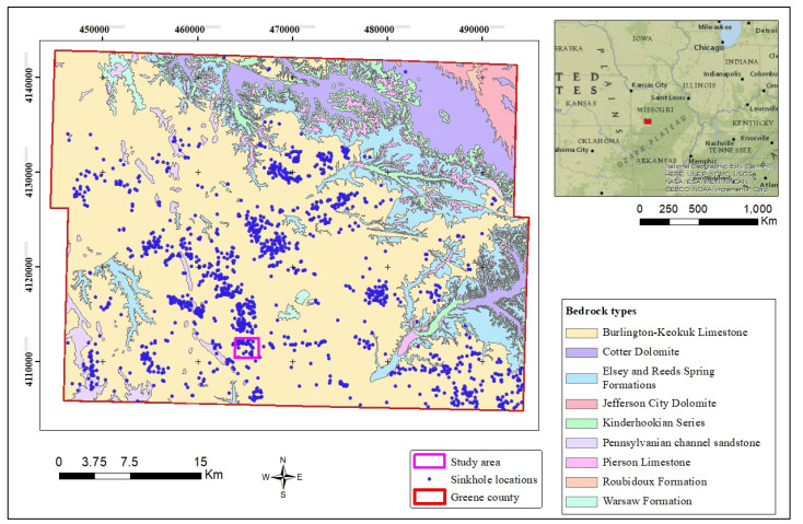
[33] | Fellows LD (1970) Geologic Map of the Galloway Quadrangle, Greene County, Missouri. Missouri Geological Survey and Water Resources. |
[34] | Orndorff RC, Weary DJ, Lagueux KM (2016) Geographic Information Systems Analysis of Geologic Controls on the Distribution on Dolines in the Ozarks of South-Central Missouri, USA. Acta Carsol 29. |
[35] | McCracken MH (1971) Structural features of Missouri. Missouri Geological Survey and Water Resources. |
[36] | Labuda TZ, Baxter AC (2001) Mapping karst conditions using 2D and 3D resistivity imaging methods. In Symposium on the Application of Geophysics to Engineering and Environmental Problems 2001. Society of Exploration Geophysicists, GTV1-GTV1. |
[37] | Loke MH (2002) Rapid 2-D Resistivity and IP inversion using the least-squares method, Geoelectrical Imaging 2D and 3D. Geotomo Softw. |
[38] |
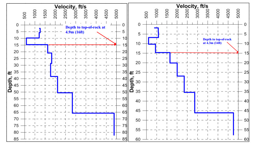
Tokeshi K, Harutoonian P, Leo CJ, et al. (2013) Use of surface waves for geotechnical engineering applications in Western Sydney. Adv Geosci 35: 37-44. doi: 10.5194/adgeo-35-37-2013
![]() |
1. | Pabalelo Sono, Bokani Nthaba, Elisha M. Shemang, Boniface Kgosidintsi, Thato Seane, An integrated use of induced polarization and electrical resistivity imaging methods to delineate zones of potential gold mineralization in the Phitshane Molopo area, Southeast Botswana, 2021, 174, 1464343X, 104060, 10.1016/j.jafrearsci.2020.104060 | |
2. | Sanaz Zarif Mahdizadeh, Ali Beitollahi, Ilnaz Zarif Mahdizadeh, Matching the experimental formula of laboratory modeling with field measurements on spherical anomalies using two-dimension electrical resistivity imaging technique, 2022, 8, 2363-6203, 3523, 10.1007/s40808-021-01290-6 | |
3. | O.O. Blake, R. Ramsook, U.C. Iyare, X.R. Moonan, R.C. Gopaul, Integrating pseudo-3D ERT and DEM to map the near-surface structures and morphology of the Piparo mud volcano, Trinidad, 2021, 194, 09269851, 104442, 10.1016/j.jappgeo.2021.104442 | |
4. | Bernadetta Pasierb, Grzegorz Gajek, Jan Urban, Wiesław Nawrocki, Integrated Geophysical and Geomorphological Studies of Caves in Calcarenite Limestones (Jaskinia pod Świecami Cave, Poland), 2024, 45, 0169-3298, 663, 10.1007/s10712-023-09821-9 | |
5. | Abdallah Basiru, Shishay T Kidanu, Sergei Rybakov, Nicholas Hasson, Moustapha Kebe, Emmanuel Osei Acheampong, Electrical Resistivity Tomography Investigation of Permafrost Conditions in a Thermokarst Site in Fairbanks, Alaska, 2024, 10, 2471-2132, 1, 10.3934/geosci.2024001 | |
6. | Rosanna Salone, Claudio De Paola, Rolando Carbonari, Francesco Rufino, Rosario Avino, Stefano Caliro, Emilio Cuoco, Alessandro Santi, Rosa Di Maio, High-resolution geoelectrical characterization and monitoring of natural fluids emission systems to understand possible gas leakages from geological carbon storage reservoirs, 2023, 13, 2045-2322, 10.1038/s41598-023-45637-8 | |
7. | Peng Bai, Dongdong Zhao, Chao Li, Shengjie Qiao, Zhengyu Liu, Arbitrary Dipole-Dipole Observation Systems and High-Precision Resistivity Imaging Algorithms for Complex Survey Areas, 2024, 62, 0196-2892, 1, 10.1109/TGRS.2024.3499978 |
Tie points of core hole and MASW data at ERT sections (S-2 & S-13) | Depth to top-of-rock | |
Core hole ties at 100 m mark of ERT S-2 | Core hole (CH-1) | 2.3 m (7.5 ft) |
ERT S-2 | 2.1 m (6.9 ft) | |
MASW-4 ties at 183 m mark of ERT S-2 | MASW-4 | 5.8 m (19 ft) |
ERT S-2 | 6.1 m (20 ft) | |
MASW-5 ties at 61 m mark of ERT S-2 | MASW-5 | 6.7 m (22 ft) |
ERT S-2 | 5.8 m (19 ft) | |
MASW-7 ties at 183 m mark of ERT S-13 | MASW-7 | 4.3 m (14 ft) |
ERT S-13 | 4.6 m (15 ft) | |
MASW-8 ties at 73 m mark of ERT S-13 | MASW-8 | 4 m (13 ft) |
ERT S-13 | 3.7 m (10 ft) |