This research explores the spillover effects in the directional movement of returns and the persistence of shocks among three prominent energy spot markets: title transfer facility for natural gas, Brent crude oil and electricity markets from monthly price data spanning January 2010 to September 2022. Methodologically, we initially employ bivariate vector autoregressive models to detect potential lagged return effects from one spot market on another. Then, we examine the impact on the conditional mean returns and volatility across these spot markets using the standard dynamic conditional correlation (DCC) model, as well as the respective asymmetric (ADCC) and flexible (FDCC) extensions. In addition, we accommodate innovative insights that include recent datasets on the COVID-19 crisis and the Ukrainian war, which constitute a new addition to the existent literature. The empirical findings confirm the significant impact of these two unprecedented moments of contemporaneous history, given that both events are substantiated by an exponential increase in prices and by a rise in volatility. However, the effect on returns was not uniform across the time series. Specifically, there was a consistent increase in volatility for natural gas and electricity from the start of 2020 until the end of 2022, while Brent oil exhibited a substantial peak only in the first half of 2020. This study also reveals that previous lagged returns within each market, particularly for Brent oil and electricity, had statistically significant effects on current returns. There was also a robust unidirectional positive spillover effect from the Brent oil market to the returns of electricity and the natural gas markets. The study also reveals the presence of a weak positive autocorrelation between natural gas and electricity returns, and positive shocks to returns had a more pronounced impact on volatility compared to negative shocks across all the time series.
Citation: Gustavo Soutinho, Vítor Miguel Ribeiro, Isabel Soares. Dynamic correlation among title transfer facility natural gas, Brent oil and electricity EPEX spot markets: Spillover effects of economic shocks on returns and volatility[J]. AIMS Energy, 2023, 11(6): 1252-1277. doi: 10.3934/energy.2023057
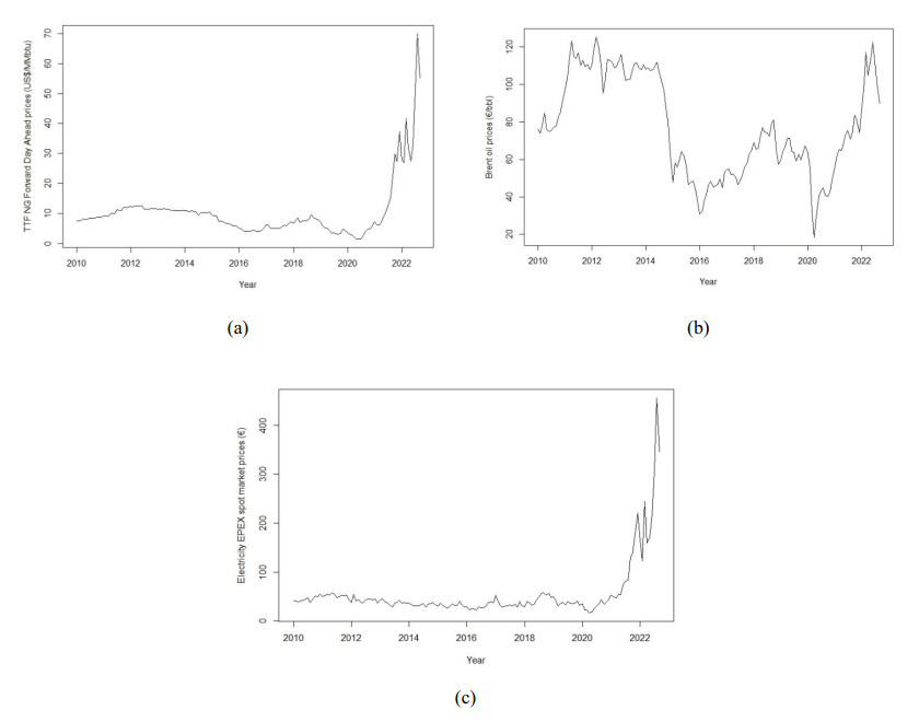
This research explores the spillover effects in the directional movement of returns and the persistence of shocks among three prominent energy spot markets: title transfer facility for natural gas, Brent crude oil and electricity markets from monthly price data spanning January 2010 to September 2022. Methodologically, we initially employ bivariate vector autoregressive models to detect potential lagged return effects from one spot market on another. Then, we examine the impact on the conditional mean returns and volatility across these spot markets using the standard dynamic conditional correlation (DCC) model, as well as the respective asymmetric (ADCC) and flexible (FDCC) extensions. In addition, we accommodate innovative insights that include recent datasets on the COVID-19 crisis and the Ukrainian war, which constitute a new addition to the existent literature. The empirical findings confirm the significant impact of these two unprecedented moments of contemporaneous history, given that both events are substantiated by an exponential increase in prices and by a rise in volatility. However, the effect on returns was not uniform across the time series. Specifically, there was a consistent increase in volatility for natural gas and electricity from the start of 2020 until the end of 2022, while Brent oil exhibited a substantial peak only in the first half of 2020. This study also reveals that previous lagged returns within each market, particularly for Brent oil and electricity, had statistically significant effects on current returns. There was also a robust unidirectional positive spillover effect from the Brent oil market to the returns of electricity and the natural gas markets. The study also reveals the presence of a weak positive autocorrelation between natural gas and electricity returns, and positive shocks to returns had a more pronounced impact on volatility compared to negative shocks across all the time series.

| [1] | Grubb M (2022) Renewables are cheaper than ever-so why are household energy bills only going up? The Conversation. Available from: https://theconversation.com/renewables-are-cheaper-than-ever-so-why-are-household-energy-bills-only-going-up-174795. |
| [2] |
Mensi W, Rehman MU, Maitra D, et al. (2021) Oil, natural gas and BRICS stock markets: Evidence of systemic risks and co-movements in the time-frequency domain. Resour Policy 72: 102062. https://doi.org/10.1016/j.resourpol.2021.102062 doi: 10.1016/j.resourpol.2021.102062

|
| [3] |
Qin Y, Hong K, Chen J, et al. (2020) Asymmetric effects of geopolitical risks on energy returns and volatility under different market conditions. Energy Econ 90: 104851. https://doi.org/10.1016/j.eneco.2020.104851 doi: 10.1016/j.eneco.2020.104851
|
| [4] |
Lee Y, Yoon SM (2020) Dynamic spillover and hedging among carbon, biofuel and oil. Energies 13: 4382. https://doi.org/10.3390/en13174382 doi: 10.3390/en13174382
|
| [5] |
Benlagha N, Karim S, Naeem MA, et al. (2022) Risk connectedness between energy and stock markets: Evidence from oil importing and exporting countries. Energy Econ 115: 106348. https://doi.org/10.1016/j.eneco.2022.106348 doi: 10.1016/j.eneco.2022.106348
|
| [6] |
Gong X, Liu Y, Wang X (2021) Dynamic volatility spillovers across oil and natural gas futures markets based on a time-varying spillover method. Int Rev Financ Anal 76: 101790. https://doi.org/10.1016/j.irfa.2021.101790 doi: 10.1016/j.irfa.2021.101790
|
| [7] |
Lovcha Y, Perez-Laborda A (2020) Dynamic frequency connectedness between oil and natural gas volatilities. Econ Model 84: 181–189. https://doi.org/10.1016/j.econmod.2019.04.008 doi: 10.1016/j.econmod.2019.04.008
|
| [8] |
Hamilton JD (1983) Oil and the macroeconomy since World War Ⅱ. J Polit Econ 91: 228–248. https://doi.org/10.1086/261140 doi: 10.1086/261140
|
| [9] |
Narayan P, Narayan S, Sharma S (2013) An analysis of commodity markets: What gain for investors? J Bank Financ 37: 3878–3889. https://doi.org/10.1016/j.jbankfin.2013.07.009 doi: 10.1016/j.jbankfin.2013.07.009
|
| [10] |
Narayan P, Amhed H, Narayan S (2015) Do momentum-based trading strategies work in the commodity futures markets? J Futures Mark 35: 868–891 https://doi.org/10.1002/fut.21685 doi: 10.1002/fut.21685
|
| [11] |
Zhao LT, Yan JL, Wang Y (2017) Empirical study of the functional changes in price discovery in the Brent crude oil market. Energy Procedia 142: 2917–2922. https://doi.org/10.1016/j.egypro.2017.12.417 doi: 10.1016/j.egypro.2017.12.417
|
| [12] |
Zhang W, He X, Nakajima T, et al. (2020) How does the spillover among natural gas, crude oil, and electricity utility stocks change over Time? Evidence from North America and Europe. Energies 13: 727. https://doi.org/10.3390/en13030727 doi: 10.3390/en13030727
|
| [13] | Adolfsen JF, Kuik F, Lis EM, et al. (2022) The impact of the war in Ukraine on euro area energy markets. ECB. Available from: https://www.ecb.europa.eu/pub/economic-bulletin/focus/2022/html/ecb.ebbox202204_01~68ef3c3dc6.en.html. |
| [14] | IEA (2023). Available from: https://www.iea.org/fuels-and-technologies/gas. |
| [15] |
Erias AE, Iglesias EM (2022) Price and income elasticity of NG demand in Europe and the effects of lockdowns due to Covid-19. Energy Strategy Rev 44: 100945. https://doi.org/10.1016/j.esr.2022.100945 doi: 10.1016/j.esr.2022.100945
|
| [16] |
Hamilton JD (2003) What is an oil shock? J Econom 113: 363–398. https://doi.org/10.1016/S0304-4076(02)00207-5 doi: 10.1016/S0304-4076(02)00207-5
|
| [17] |
Emery GW, Liu WQ (2002) An analysis of the relationship between electricity and natural-gas futures prices. J Futures Mark 22: 95–122. https://doi.org/10.1002/fut.2209 doi: 10.1002/fut.2209
|
| [18] |
Woo C, Olson A, Horowitz I, et al. (2006) Bi-directional causality in California's electricity and natural-gas markets. Energy Policy 34: 2060–2070. https://doi.org/10.1016/j.enpol.2005.02.016 doi: 10.1016/j.enpol.2005.02.016
|
| [19] |
Serletis A, Shahmoradi A (2006) Measuring and testing natural gas and electricity markets volatility: Evidence from Alberta's deregulated markets. Stud Nonlinear Dyn Econ 10: 1341. https://doi.org/10.2202/1558-3708.1341 doi: 10.2202/1558-3708.1341
|
| [20] |
Arouri MEH, Jouini J, Nguyen DK (2011) Volatility spillovers between oil prices and stock sector returns: Implications for portfolio management. J Int Money Finance 30: 1387–1405. https://doi.org/10.1016/j.jimonfin.2011.07.008 doi: 10.1016/j.jimonfin.2011.07.008
|
| [21] |
Arouri MEH, Lahiani A, Nguyen DK (2011) Return and volatility transmission between world oil prices and stock markets of the GCC countries. Econ Model 28: 1815–1825. https://doi.org/10.1016/j.econmod.2011.03.012 doi: 10.1016/j.econmod.2011.03.012
|
| [22] |
Ewing BT, Malik F, Ozfidan O (2002) Volatility transmission in the oil and natural gas markets. Energy Econ 24: 525–538. https://doi.org/10.1016/S0140-9883(02)00060-9 doi: 10.1016/S0140-9883(02)00060-9
|
| [23] |
Oberndorfer U (2009) Energy prices, volatility, and the stock market: Evidence from the Eurozone. Energy Policy 37: 5787–5795. https://doi.org/10.1016/j.enpol.2009.08.043 doi: 10.1016/j.enpol.2009.08.043
|
| [24] |
Oberndorfer U (2009) EU emission allowances and the stock market: Evidence from the electricity industry. Ecol Econ 68: 1116–1129. https://doi.org/10.1016/j.ecolecon.2008.07.026 doi: 10.1016/j.ecolecon.2008.07.026
|
| [25] |
Luo C, Wu D (2016) Environment and economic risk: An analysis of carbon emission market and portfolio management. Environ Res 149: 297–301. https://doi.org/10.1016/j.envres.2016.02.007 doi: 10.1016/j.envres.2016.02.007
|
| [26] |
Shehzad K, Xiaoxing L, Kazouz H (2020) COVID-19's disasters are perilous than global financial crisis: a rumor or fact? Finance Res Lett 36: 101669. https://doi.org/10.1016/j.frl.2020.101669 doi: 10.1016/j.frl.2020.101669
|
| [27] |
Conlon T, McGee R (2020) Safe haven or risky hazard? Bitcoin during the COVID-19 bear market. Finance Res Lett 35: 101607. https://doi.org/10.1016/j.frl.2020.101607 doi: 10.1016/j.frl.2020.101607
|
| [28] |
Conlon T, Corbet S, McGee RJ (2020) Are cryptocurrencies a safe haven for equity markets? An international perspective from the COVID-19 pandemic. Res Int Bus Finance 54: 101248. https://doi.org/10.1016/j.ribaf.2020.101248 doi: 10.1016/j.ribaf.2020.101248
|
| [29] |
Goodell JW (2020) Covid-19 and finance: Agendas for future research. Finance Res Lett 35: 101512. https://doi.org/10.1016/j.frl.2020.101512 doi: 10.1016/j.frl.2020.101512
|
| [30] |
Goutte S, Péran T, Porcher T (2020) The role of economic structural factors in determining pandemic mortality rates: Evidence from the COVID-19 outbreak in france. Res Int Bus Finance 54:101281. https://doi.org/10.1016/j.ribaf.2020.101281 doi: 10.1016/j.ribaf.2020.101281
|
| [31] |
Chaaya C, Thambi VD, Sabuncu Ö, et al. (2022) Ukraine–Russia crisis and its impacts on the mental health of Ukrainian young people during the COVID-19 pandemic. Ann Med Surg 79: 104033. https://doi.org/10.1016/j.amsu.2022.104033 doi: 10.1016/j.amsu.2022.104033
|
| [32] |
Roy A, Soni A, Deg S (2023) A wavelet-based methodology to compare the impact of pandemic versus Russia–Ukraine conflict on crude oil sector and its interconnectedness with other energy and non-energy markets. Energy Econ 124: 106830. https://doi.org/10.1016/j.eneco.2023.106830 doi: 10.1016/j.eneco.2023.106830
|
| [33] | European Commission (2022) Quarterly report on European gas markets. Market Observatory for Energy DG Energy. Available from: https://energy.ec.europa.eu/system/files/2023-05/Quarterly%20Report%20on%20European%20Gas%20Markets%20report%20Q4%202022.pdf. |
| [34] |
Inshakov OV, Bogachkova LY, Popkova EG (2019) The transformation of the global energy markets and the problem of ensuring the sustainability of their development. Lect Notes Netw Syst 44: 135–148. https://doi.org/10.1007/978-3-319-90966-0_10 doi: 10.1007/978-3-319-90966-0_10
|
| [35] |
Liu Y, Yu L, Yang C, et al. (2021) Heterogeneity of the impact of geopolitical events on energy trade: an empirical study based on regression discontinuity design. Front Environ Sci 9: 322. https://doi.org/10.3389/fenvs.2021.722910 doi: 10.3389/fenvs.2021.722910
|
| [36] |
Gong X, Sun Y, Du Z (2022) Geopolitical risk and China's oil security. Energy Policy 163: 112856. https://doi.org/10.1016/j.enpol.2022.112856 doi: 10.1016/j.enpol.2022.112856
|
| [37] |
Zhang Z, He M, Zhang Y, et al. (2022) Geopolitical risk trends and crude oil price predictability. Energy 258: 124824. https://doi.org/10.1016/j.energy.2022.124824 doi: 10.1016/j.energy.2022.124824
|
| [38] |
Dutta A, Dutta P (2022) Geopolitical risk and renewable energy asset prices: Implications for sustainable development. Renew Energy 196: 518–525. https://doi.org/10.1016/j.renene.2022.07.029 doi: 10.1016/j.renene.2022.07.029
|
| [39] |
Su CW, Khan K, Umar M, et al. (2021) Does renewable energy redefine geopolitical risks? Energy Policy 158. https://doi.org/10.1016/j.enpol.2021.112566 doi: 10.1016/j.enpol.2021.112566
|
| [40] |
Ali F, Suri P, Kaur T, et al. (2022) Modelling time-varying volatility using GARCH models: Evidence from the Indian stock market. F1000Res 27: 1098. https://doi.org/10.12688/f1000research.124998.2 doi: 10.12688/f1000research.124998.2
|
| [41] |
Nandy S, Chattopadhyay AK (2019) Indian stock market volatility: A study of inter-linkages and spillover effects. J Emerg Mark Finance 18: 183–212. https://doi.org/10.1177/0972652719846321 doi: 10.1177/0972652719846321
|
| [42] |
Jebabli I, Kouaissah N, Arouri M (2022) Volatility spillovers between stock and energy markets during crises: A comparative assessment between the 2008 global financial crisis and the COVID-19 pandemic crisis. Finance Res Lett 46: 102363. https://doi.org/10.1016/j.frl.2021.102363 doi: 10.1016/j.frl.2021.102363
|
| [43] |
Gharib C, Mefteh-Wali S, Jabeur SB (2021) The bubble contagion effect of COVID-19 outbreak: Evidence from crude oil and gold markets. Finance Res Lett 38: 101703. https://doi.org/10.1016/j.frl.2020.101703 doi: 10.1016/j.frl.2020.101703
|
| [44] |
Mensi W, Sensoy A, Vo XV, et al. (2020) Impact of COVID-19 outbreak on asymmetric multifractality of gold and oil prices. Resour Policy 69: 101829. https://doi.org/10.1016/j.resourpol.2020.101829 doi: 10.1016/j.resourpol.2020.101829
|
| [45] |
Wen F, Tong X, Ren X (2022) Gold or bitcoin, which is the safe haven during the COVID-19 pandemic? Int Rev Financ Anal 81: 102121. https://doi.org/10.1016/j.irfa.2022.102121 doi: 10.1016/j.irfa.2022.102121
|
| [46] |
Elsayed AH, Gozgor G, Lau CKM (2022) Risk transmissions between bitcoin and traditional financial assets during the COVID-19 era: The role of global uncertainties. Int Rev Financ Anal 81: 102069. https://doi.org/10.1016/j.irfa.2022.102069 doi: 10.1016/j.irfa.2022.102069
|
| [47] |
Dritsaki C (2017) An empirical evaluation in GARCH volatility modeling: Evidence from the Stockholm stock exchange. J math financ 7: 366–390. https://doi.org/10.4236/jmf.2017.72020 doi: 10.4236/jmf.2017.72020
|
| [48] |
Engle RF (1982) Autoregressive conditional heteroscedasticity with estimates of the variance of UK inflation. Econometrica 50: 987–1007. https://doi.org/10.2307/1912773 doi: 10.2307/1912773
|
| [49] |
Bollerslev T (1986) Generalized autoregressive conditional heteroskedasticity. J Econom 31: 307–327. https://doi.org/10.1016/0304-4076(86)90063-1 doi: 10.1016/0304-4076(86)90063-1
|
| [50] |
Sarwar S, Shahbaz M, Anwar A (2019) The importance of oil assets for portfolio optimization: the analysis of firm level stocks. Energy Econ 78: 217–234. https://doi.org/10.1016/j.eneco.2018.11.021 doi: 10.1016/j.eneco.2018.11.021
|
| [51] |
Afzal F, Haiying P, Afzal F, et al. (2021) Value-at-risk analysis for measuring stochastic volatility of stock returns: using GARCH-based dynamic donditional correlation Model. SAGE Open 11. https://doi.org/10.1177/21582440211005758 doi: 10.1177/21582440211005758
|
| [52] | Black F (1976) Studies in stock price volatility changes of the nominal excess return on stocks. Proceedings of the business and economics statistics section, American statistical association 81: 177–181. |
| [53] | Ari Y (2020) Volatility transmission model using DCC-GARCH representation. In: Samet Evci, Anshuman Sharma. Studies at the Crossroads of Management & Economics, London: IJOPEC, 237–250. |
| [54] | Engle RF (2002) Dynamic conditional correlation: A simple class of multivariate generalized autoregressive conditional heteroskedasticity models. J Bus Econ Stat 20: 339–350. https://www.jstor.org/stable/1392121 |
| [55] |
Bollerslev T (1990) Modelling the coherence in short-run nominal exchange rates: A multivariate generalized ARCH model. Rev Econ Stat 72: 498–505. https://doi.org/10.2307/2109358 doi: 10.2307/2109358
|
| [56] |
Cappiello L, Engle RF, Sheppard K (2006) Asymmetric dynamics in the correlations of global equity and bond returns. J Financ Econ 4: 537–572. https://doi.org/10.1093/jjfinec/nbl005 doi: 10.1093/jjfinec/nbl005
|
| [57] |
Billio M, Caporin M, Gobbo M (2006) Flexible dynamic conditional correlation multivariate GARCH models for asset allocation. Appl Financ Econ Lett 2: 123–130. https://doi.org/10.1080/17446540500428843 doi: 10.1080/17446540500428843
|
| [58] |
Celik S (2012) The more contagion effect on emerging markets: the evidence of DCC-GARCH model. Econ Modell 29: 1946–1959. https://doi.org/10.1016/j.econmod.2012.06.011 doi: 10.1016/j.econmod.2012.06.011
|
| [59] | Duca JV (2023) Subprime mortgage crisis. Federal Reserve History. Available from: https://www.federalreservehistory.org/essays/subprime-mortgage-crisis. |
| [60] | Nasdaq Data Link (2023). Available from: https://data.nasdaq.com/data/ODA/PNGASEU_USD-natural-gas-netherlands-ttf-natural-gas-forward-day-ahead-us-per-million-metric-british-thermal-unit. |
| [61] | US Energy Information Administration (EIA), 2023. Available from: https://www.eia.gov/dnav/pet/hist/LeafHandler.ashx?n = PET & s = RBRTE & f = M. |
| [62] | Energy-Charts (2023). Available from: https://www.energy-charts.info/index.html?l = en & c = DE. |
| [63] | EEX (2023). Available from: https://www.powernext.com/spot-market-data. |
| [64] | Manescu C, Van Robays I (2014) Forecasting the brent oil price addressing time-variation in forecast performance. European Central Bank. Available from: https://www.ecb.europa.eu/pub/pdf/scpwps/ecbwp1735.pdf. |
| [65] |
Jarque CM, Bera AK (1980) Efficient tests for normality, homoscedasticity and serial independence of regression residuals. Econ Lett 6: 255–259. https://doi.org/10.1016/0165-1765(80)90024-5 doi: 10.1016/0165-1765(80)90024-5
|
| [66] |
Ljung G, Box G (1978) On a Measure of a lack of fit in time series models. Biometrika 65: 297–303. https://doi.org/10.1093/biomet/65.2.297 doi: 10.1093/biomet/65.2.297
|
| [67] | PennState-Eberly College of Science (2023) STAT 509, Design and Analysis of Clinical Trials. Available from: https://online.stat.psu.edu/stat509/lesson/18/18.1. |
| [68] | Greene WH (2017) Econometric Analysis. Pearson. |
| [69] |
Dickey DA, Fuller WA (1979) Distribution of the estimators for autoregressive time series with a unit root. J AM STAT ASSOC 74: 427–431. https://doi.org/10.2307/2286348 doi: 10.2307/2286348
|
| [70] |
Cragg JG (1983) More efficient estimation in the presence of heteroskedasticity of unknown form. Econometrica 51: 751–764. https://doi.org/10.2307/1912156 doi: 10.2307/1912156
|
| [71] | Brooks, C (2014) Introductory econometrics for finance, Cambridge: Cambridge University Press. |
| [72] |
Dutta A, Bouri E, Noor MH (2018) Return and volatility linkages between CO2 emission and clean energy stock prices. Energy 164: 803–810. https://doi.org/10.1016/j.energy.2018.09.055 doi: 10.1016/j.energy.2018.09.055
|
| [73] |
Ahmad W (2017) On the dynamic dependence and investment performance of crude oil and clean energy stocks. Res Int Bus Finance 42: 376–389. https://doi.org/10.1016/j.ribaf.2017.07.140 doi: 10.1016/j.ribaf.2017.07.140
|
| [74] |
Ahmad W, Sadorsky P, Sharma A (2018) Optimal hedge ratios for clean energy equities. Econ Modell 72: 278–295. https://doi.org/10.1016/j.econmod.2018.02.008 doi: 10.1016/j.econmod.2018.02.008
|
| [75] |
Granger C (1969) Investigating causal relations by econometric models and cross-spectral Methods. Econometrica 37: 424–438. https://doi.org/10.2307/1912791 doi: 10.2307/1912791
|
| [76] |
Troster V (2018) Testing for granger-causality in quantiles. Econom Rev 7: 850–866. https://doi.org/10.1080/07474938.2016.1172400 doi: 10.1080/07474938.2016.1172400
|
| [77] |
Engle R, Sheppard K (2001) GARCH 101: The use of ARCH/GARCH models in applied econometrics. J Econ Perspect 15: 157–168. https://doi.org/10.1257/jep.15.4.157 doi: 10.1257/jep.15.4.157
|
| [78] | Alexander C (2008) Market Risk Analysis: Pricing, Hedging and Trading Financial Instruments. Hoboken: John Wiley & Sons Ltd. |


Figures(4) / Tables(4)

Gustavo Soutinho, Vítor Miguel Ribeiro, Isabel Soares. Dynamic correlation among title transfer facility natural gas, Brent oil and electricity EPEX spot markets: Spillover effects of economic shocks on returns and volatility[J]. AIMS Energy, 2023, 11(6): 1252-1277. doi: 10.3934/energy.2023057


 DownLoad: