Prediction of the equivalent circulation density using machine learning algorithms based on real-time data

Abdelrahman Kandil; Samir Khaled; Taher Elfakharany; Abdelrahman Kandil; Samir Khaled; Taher Elfakharany

doi:10.3934/energy.2023023

AIMS Energy

2023, Volume 11, Issue 3: 425-453. doi: 10.3934/energy.2023023

Previous Article Next Article

Research article

Prediction of the equivalent circulation density using machine learning algorithms based on real-time data

1.
Department of Petroleum Engineering, Faculty of Engineering and Technology, Future University in Egypt (FUE), Cairo 11835, Egypt
2.
Department of Mining and Petroleum Engineering, Faculty of Engineering, Al-Azhar University, Cairo 11835, Egypt

Received: 28 January 2023 Revised: 04 April 2023 Accepted: 22 April 2023 Published: 08 May 2023

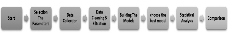
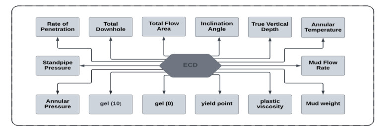
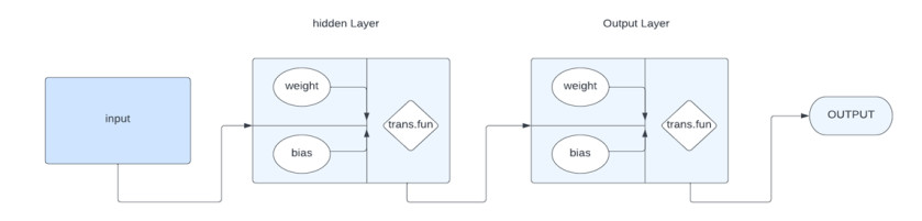
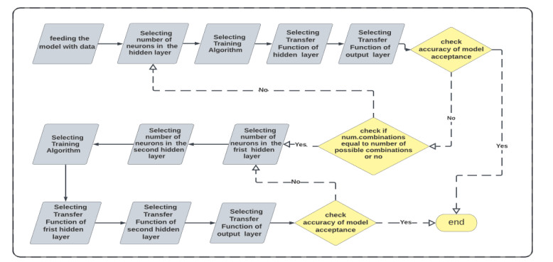
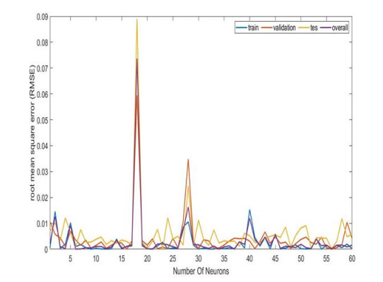
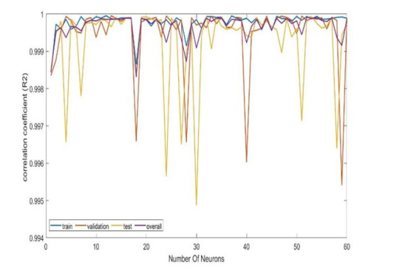
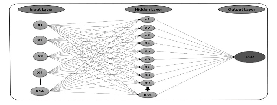
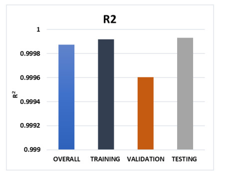
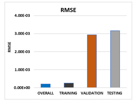
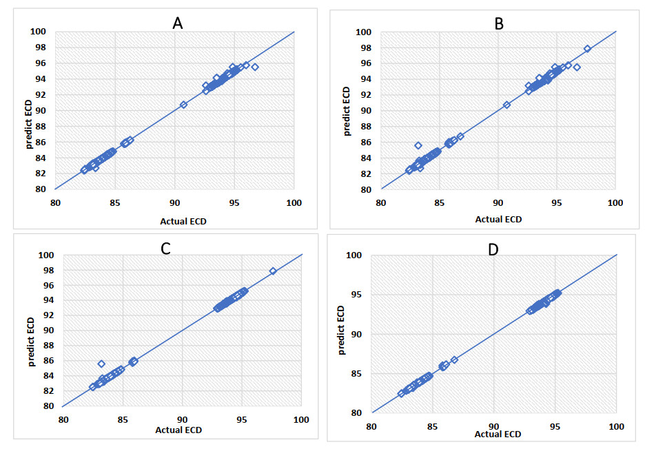
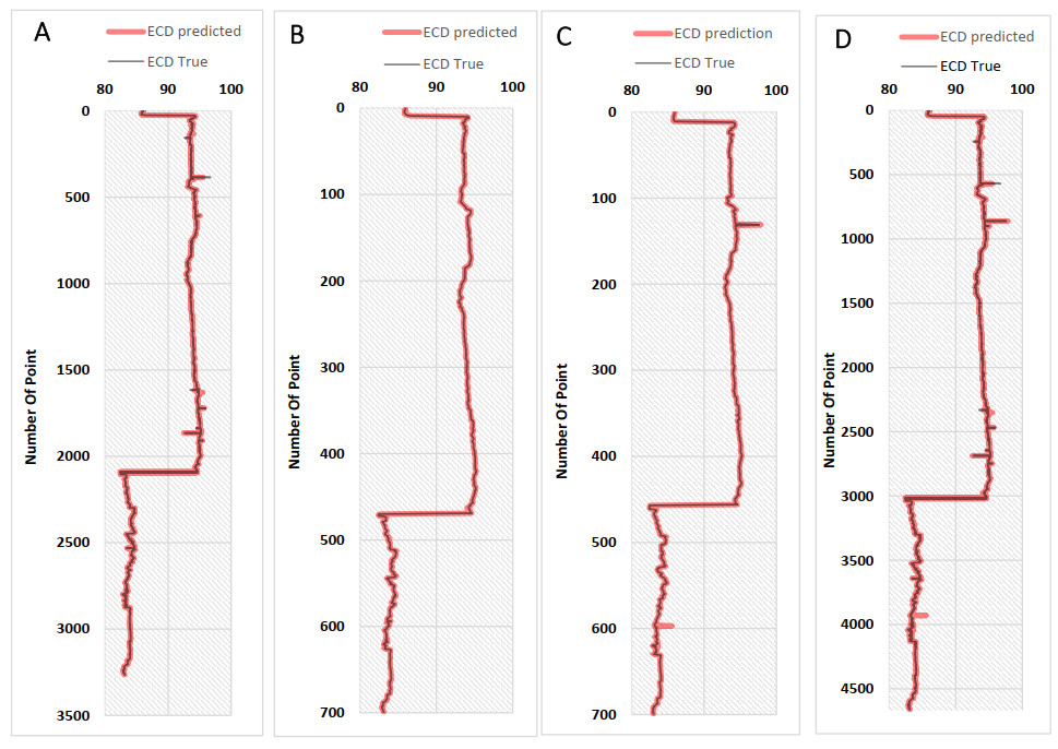
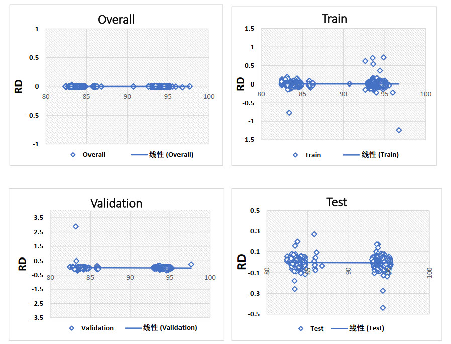
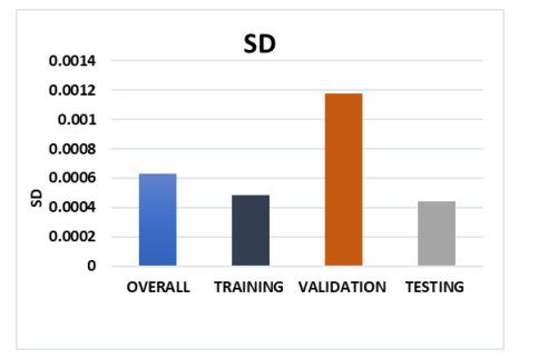
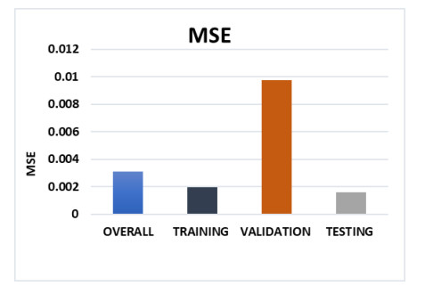
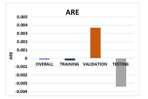
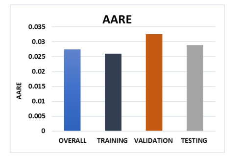
Equivalent circulation density (ECD) is one of the most important parameters that should be considered while designing drilling programs. With increasing the wells' deep, offshore hydrocarbon extraction, the costly daily rate of downhole measurements, operating restrictions, and the fluctuations in the global market prices, it is necessary to reduce the non-productive time and costs associated with hole problems resulting from ignoring and incorrect evaluation of ECD. Therefore, optimizing ECD and selecting the best drilling parameters are curial tasks in such operations. The main objective of this work is to predict ECD using three machine learning algorithms: an artificial neural network (ANN) with a Levenberg-Marquardt backpropagation algorithm, a K neighbors regressor (knn), and a passive aggressive regressor (par). These models are based on 14 critical operation parameters that have been provided by downhole sensors during drilling operations such as annular pressure, annular temperature, and rate of penetration, etc. In the study, 4663 data points were selected and included, where 80% to 85% of the data set has been used for training and validation according to the algorithm, and the remaining data points were reserved for testing. In addition, several statistical tests were used to evaluate the accuracy of the models, including root mean square error (RMSE), correlation coefficient (R²), and mean squared error (MSE). The results of the developed models show various consistencies and accuracy, while the ANN shows a high accuracy with an R² of nearly 0.999 for the training, validation, and testing, as well as the overall of them. The RMSE is 0.000211, 0.000253, 0.00293, and 0.00315 for overall, training, validation, and testing, respectively. This work expands the use of artificial intelligence in the gas and oil industry. The developed ANN model is more flexible in response to challenges, reduces dependence on humans, and thus, reduces the chance of human omission, as well as increasing the efficiency of operations.
- Equivalent circulation density (ECD),
- artificial intelligence (AI),
- drilling wells,
- artificial neural networks (ANN),
- real-time data
Citation: Abdelrahman Kandil, Samir Khaled, Taher Elfakharany. Prediction of the equivalent circulation density using machine learning algorithms based on real-time data[J]. AIMS Energy, 2023, 11(3): 425-453. doi: 10.3934/energy.2023023

Related Papers:

Abstract

Equivalent circulation density (ECD) is one of the most important parameters that should be considered while designing drilling programs. With increasing the wells' deep, offshore hydrocarbon extraction, the costly daily rate of downhole measurements, operating restrictions, and the fluctuations in the global market prices, it is necessary to reduce the non-productive time and costs associated with hole problems resulting from ignoring and incorrect evaluation of ECD. Therefore, optimizing ECD and selecting the best drilling parameters are curial tasks in such operations. The main objective of this work is to predict ECD using three machine learning algorithms: an artificial neural network (ANN) with a Levenberg-Marquardt backpropagation algorithm, a K neighbors regressor (knn), and a passive aggressive regressor (par). These models are based on 14 critical operation parameters that have been provided by downhole sensors during drilling operations such as annular pressure, annular temperature, and rate of penetration, etc. In the study, 4663 data points were selected and included, where 80% to 85% of the data set has been used for training and validation according to the algorithm, and the remaining data points were reserved for testing. In addition, several statistical tests were used to evaluate the accuracy of the models, including root mean square error (RMSE), correlation coefficient (R²), and mean squared error (MSE). The results of the developed models show various consistencies and accuracy, while the ANN shows a high accuracy with an R² of nearly 0.999 for the training, validation, and testing, as well as the overall of them. The RMSE is 0.000211, 0.000253, 0.00293, and 0.00315 for overall, training, validation, and testing, respectively. This work expands the use of artificial intelligence in the gas and oil industry. The developed ANN model is more flexible in response to challenges, reduces dependence on humans, and thus, reduces the chance of human omission, as well as increasing the efficiency of operations.

References

[1]	Hansen KV (1993) Neural networks for primary reflection identification. SEG Technical Program Expanded Abstracts, 242–245. https://doi.org/10.1190/1.1822450 doi: 10.1190/1.1822450
[2]	Kononov A, Gisolf D, Verschuur E (2007) Application of neural networks to travel-times computation. 2007 SEG Annual Meeting, San Antonio, Texas, SEG-2007-1785. Available from: https://onepetro.org/SEGAM/proceedings-abstract/SEG07/All-SEG07/SEG-2007-1785/95760.
[3]	Syed FI, AlShamsi A, Dahaghi AK, et al. (2022) Application of ML & AI to model petrophysical and geomechanical properties of shale reservoirs—A systematic literature review. Petroleum 8: 158–166. https://doi.org/10.1016/j.petlm.2020.12.001 doi: 10.1016/j.petlm.2020.12.001
[4]	Arehart RA (1990) Drill-bit diagnosis with neural networks. SPE Comput Appl 2: 24–28. https://doi.org/10.2118/19558-PA doi: 10.2118/19558-PA
[5]	Moran D, Ibrahim H, Purwanto A, et al. (2010) Sophisticated ROP prediction technologies based on neural network delivers accurate drill time results. IADC/SPE Asia Pacific Drilling Technology Conference and Exhibition, SPE-132010-MS, OnePetro. https://doi.org/10.2118/132010-MS
[6]	Sprunger C, Muther T, Syed FI, et al. (2022) State of the art progress in hydraulic fracture modeling using AI/ML techniques. Model Earth Syst Environ 8: 1–13. https://doi.org/10.1007/s40808-021-01111-w doi: 10.1007/s40808-021-01111-w
[7]	Denney D (2000) Artificial neural networks identify restimulation candidates. J Pet Technol 52: 44–45. https://doi.org/10.2118/0200-0044-JPT doi: 10.2118/0200-0044-JPT
[8]	Syed FI, Alshamsi M, Dahaghi AK, et al. (2022) Artificial lift system optimization using machine learning applications. Petroleum 8: 219–226. https://doi.org/10.1016/j.petlm.2020.08.003 doi: 10.1016/j.petlm.2020.08.003
[9]	Yang H-S, Kim N-S (1996) Determination of rock properties by accelerated neural network. 2nd North American Rock Mechanics Symposium, Montreal, Quebec, Canada, ARMA-96-1567, OnePetro. Available from: https://onepetro.org/ARMANARMS/proceedings/NARMS96/All-NARMS96/ARMA-96-1567/130834.
[10]	Kohli A, Arora P (2014) Application of artificial neural networks for well logs. European Assoc Geosci Eng. https://doi.org/10.3997/2214-4609-pdb.395.IPTC-17475-MS doi: 10.3997/2214-4609-pdb.395.IPTC-17475-MS
[11]	Syed FI, Alnaqbi S, Muther T, et al. (2022) Smart shale gas production performance analysis using machine learning applications. Pet Res 7: 21–31. https://doi.org/10.1016/j.ptlrs.2021.06.003 doi: 10.1016/j.ptlrs.2021.06.003
[12]	Syed FI, Muther T, Dahaghi AK, et al. (2021) AI/ML assisted shale gas production performance evaluation. J Petrol Explor Prod Technol 11: 3509–3519. https://doi.org/10.1007/s13202-021-01253-8 doi: 10.1007/s13202-021-01253-8
[13]	Yehia T, Khattab H, Tantawy M, et al. (2022) Improving the shale gas production data using the angular-based outlier detector machine learning algorithm. J Univ Shanghai Sci Technol 24: 152–172. Available from: https://jusst.org/wp-content/uploads/2022/08/Improving-the-Shale-Gas-Production-Data-Using-the.pdf.
[14]	Yehia T, Khattab H, Tantawy M, et al. (2022) Removing the outlier from the production data for the decline curve analysis of shale gas reservoirs: A comparative study using machine learning. ACS Omega 7: 32046–32061. https://doi.org/10.1021/acsomega.2c03238 doi: 10.1021/acsomega.2c03238
[15]	Yehia T, Wahba A, Mostafa S, et al. (2022) Suitability of different machine learning outlier detection algorithms to improve shale gas production data for effective decline curve analysis. Energies 15: 8835. https://doi.org/10.3390/en15238835 doi: 10.3390/en15238835
[16]	Haciislamoglu M (1994) Practical pressure loss predictions in realistic annular geometries. SPE Annual Technical Conference and Exhibition, OnePetro. https://doi.org/10.2118/28304-MS doi: 10.2118/28304-MS
[17]	Gamal H, Abdelaal A, Elkatatny S (2021) Machine learning models for equivalent circulating density prediction from drilling data. ACS Omega 6: 27430–27442. https://doi.org/10.1021/acsomega.1c04363 doi: 10.1021/acsomega.1c04363
[18]	Arshad U, Jain B, Ramzan M, et al. (2015) Engineered solution to reduce the impact of lost circulation during drilling and cementing in rumaila field, Iraq. International Petroleum Technology Conference, Doha, Qatar, OnePetro. https://doi.org/10.2523/IPTC-18245-MS
[19]	Al-Rubaii MM, Al-Nassar FY, Al-Harbi S (2022) A new real time prediction of equivalent circulation density from drilling surface parameters without using pwd tool. SPE Symposium: Unconventionals in the Middle East - From Exploration to Development Optimisation, Manama, Bahrain, SPE-209945-MS, OnePetro. https://doi.org/10.2118/209945-MS
[20]	Marsh HN (1931) Properties and treatment of rotary mud. Transac AIME 92: 234–251. https://doi.org/10.2118/931234-G doi: 10.2118/931234-G
[21]	Zhang H, Sun T, Gao D, et al. (2013) A new method for calculating the equivalent circulating density of drilling fluid in deepwater drilling for oil and gas. Chem Technol Fuels Oils 49: 430–438. https://doi.org/10.1007/s10553-013-0466-0 doi: 10.1007/s10553-013-0466-0
[22]	Abdelgawad KZ, Elzenary M, Elkatatny S, et al. (2019) New approach to evaluate the equivalent circulating density (ECD) using artificial intelligence techniques. J Petrol Explor Prod Technol 9: 1569–1578. https://doi.org/10.1007/s13202-018-0572-y doi: 10.1007/s13202-018-0572-y
[23]	Ataga E, Ogbonna J (2012) Accurate estimation of equivalent circulating density during high pressure high temperature (HPHT) drilling operations. Nigeria Annual International Conference and Exhibition, OnePetro. https://doi.org/10.2118/162972-MS
[24]	Erge O, Vajargah AK, Ozbayoglu ME, et al. (2016) Improved ECD prediction and management in horizontal and extended reach wells with eccentric drillstrings. IADC/SPE Drilling Conference and Exhibition, OnePetro. https://doi.org/10.2118/178785-MS
[25]	Rommetveit R, Ødegård SI, Nordstrand C, et al. (2010) Drilling a challenging HPHT well utilizing an advanced ECD management system with decision support and real time simulations. IADC/SPE Drilling Conference and Exhibition, New Orleans, Louisiana, USA, February 2010, SPE-128648-MS. https://doi.org/10.2118/128648-MS
[26]	Hoberock LL, Thomas DC, Nickens HV (1982) Here's how compressibility and temperature affect bottom-hole mud pressure. Oil Gas J 80: 12. Available from: https://www.osti.gov/biblio/5213477.
[27]	Peters EJ, Chenevert ME, Zhang C (1990) A model for predicting the density of oil-based muds at high pressures and temperatures. SPE Drilling Eng 5: 141–148. https://doi.org/10.2118/18036-PA doi: 10.2118/18036-PA
[28]	Bybee K (2009) Equivalent-circulating-density fluctuation in extended-reach drilling. J Pet Technol 61: 64–67. https://doi.org/10.2118/0209-0064-JPT doi: 10.2118/0209-0064-JPT
[29]	Hemphill T, Ravi K, Bern PA, et al. (2008) A simplified method for prediction of ECD increase with drillpipe rotation. SPE Annual Technical Conference and Exhibition, OnePetro. https://doi.org/10.2118/115378-MS
[30]	Ahmed R, Enfis M, Miftah-El-Kheir H, et al. (2010) The effect of drillstring rotation on equivalent circulation density: Modeling and analysis of field measurements. SPE Annual Technical Conference and Exhibition, Florence, Italy, SPE-135587-MS, OnePetro. https://doi.org/10.2118/135587-MS
[31]	Costa SS, Stuckenbruck S, Fontoura SA, et al. (2008) Simulation of transient cuttings transportation and ECD in wellbore drilling. Europec/EAGE Conference and Exhibition, OnePetro. https://doi.org/10.2118/113893-MS
[32]	Baranthol C, Alfenore J, Cotterill MD, et al. (1995) Determination of hydrostatic pressure and dynamic ecd by computer models and field measurements on the directional HPHT Well 22130C-13. SPE/IADC Drilling Conference, Amsterdam, Netherlands, OnePetro. https://doi.org/10.2118/29430-MS
[33]	Osman EA, Aggour MA (2003) Determination of drilling mud density change with pressure and temperature made simple and accurate by ANN. Middle East Oil Show, OnePetro. https://doi.org/10.2118/81422-MS
[34]	Harris O, Osisanya S (2005) SPE 97018 evaluation of equialent circulating density of drilling fluids under high-pressure/high-temperature conditions. SPE Annual Technical Conference and Exhibition, Dallas, Texas, SPE-97018-MS. https://doi.org/10.2118/97018-MS
[35]	Elzenary M, Elkatatny S, Abdelgawad KZ, et al. (2018) New technology to evaluate equivalent circulating density while drilling using artificial intelligence. SPE Kingdom of Saudi Arabia Annual Technical Symposium and Exhibition, OnePetro. https://doi.org/10.2118/192282-MS
[36]	Ahmadi MA (2016) Toward reliable model for prediction drilling fluid density at wellbore conditions: A LSSVM model. Neurocomputing 211: 143–149. https://doi.org/10.1016/j.neucom.2016.01.106 doi: 10.1016/j.neucom.2016.01.106
[37]	Ahmadi MA, Shadizadeh SR, Shah K, et al. (2018) An accurate model to predict drilling fluid density at wellbore conditions. Egyptian J Pet 27: 1–10. https://doi.org/10.1016/j.ejpe.2016.12.002 doi: 10.1016/j.ejpe.2016.12.002
[38]	Rahmati AS, Tatar A (2019) Application of Radial Basis Function (RBF) neural networks to estimate oil field drilling fluid density at elevated pressures and temperatures. Oil Gas Sci Technol—Rev IFP Energies nouvelles 74: 50. https://doi.org/10.2516/ogst/2019021 doi: 10.2516/ogst/2019021
[39]	Alkinani HH, Al-Hameedi AT, Dunn-Norman S, et al. (2019) Data-Driven neural network model to predict equivalent circulation density ECD. SPE Gas & Oil Technology Showcase and Conference, Dubai, UAE, OnePetro. https://doi.org/10.2118/198612-MS
[40]	Alsaihati A, Elkatatny S, Abdulraheem A (2020) Real-time prediction of equivalent circulation density for horizontal wells using intelligent machines. ACS Omega 6: 934–942. https://doi.org/10.1021/acsomega.0c05570 doi: 10.1021/acsomega.0c05570
[41]	Saeedi A, Camarda KV, Liang J-T (2007) Using neural networks for candidate selection and well performance prediction in water-shutoff treatments using polymer gels—A field-case study. SPE Prod Oper 22: 417–424. https://doi.org/10.2118/101028-PA doi: 10.2118/101028-PA
[42]	Vickers NJ (2017) Animal communication: When I'm calling you, will you answer too? Curr Biol 27: R713–R715. https://doi.org/10.1016/j.cub.2017.05.064 doi: 10.1016/j.cub.2017.05.064

Reader Comments

Your name:*

Email:*
© 2023 the Author(s), licensee AIMS Press. This is an open access article distributed under the terms of the Creative Commons Attribution License (http://creativecommons.org/licenses/by/4.0)