Property assessment of Peterson's mutual exclusion algorithms

Libero Nigro; Franco Cicirelli; Libero Nigro; Franco Cicirelli

doi:10.3934/aci.2024005

Applied Computing and Intelligence

2024, Volume 4, Issue 1: 66-92. doi: 10.3934/aci.2024005

Previous Article Next Article

Research article

Property assessment of Peterson's mutual exclusion algorithms

Libero Nigro ^{1
,
,},
Franco Cicirelli ²

1.
University of Calabria, DIMES, 87036 Rende, Italy
2.
CNR - National Research Council of Italy - Institute for High Performance Computing and Networking (ICAR) - 87036 Rende, Italy

Academic Editor: Pasi Fränti

Received: 22 July 2024 Revised: 16 August 2024 Accepted: 21 August 2024 Published: 28 August 2024

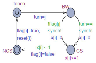
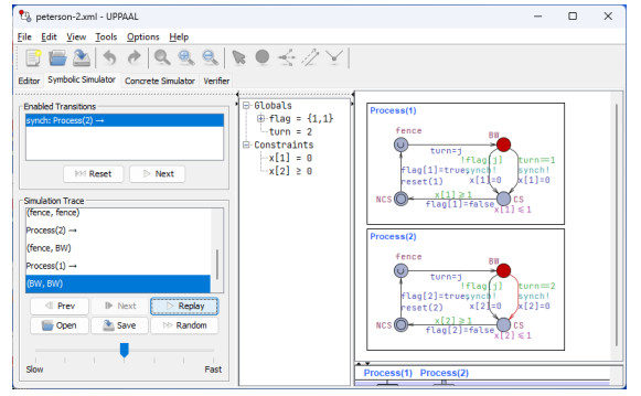
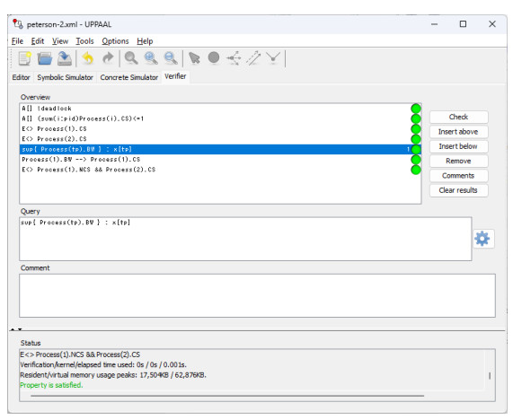
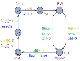
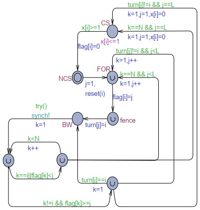
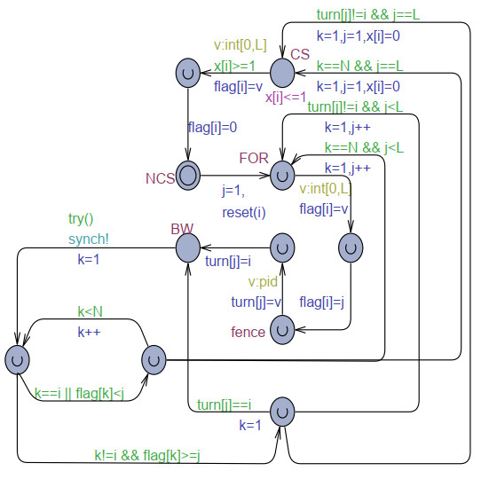
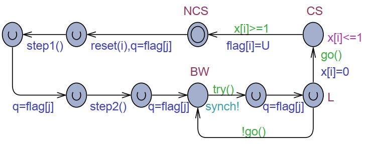
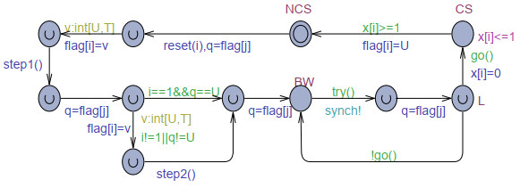
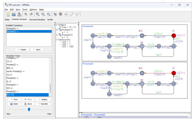
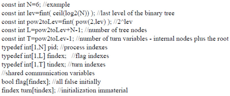
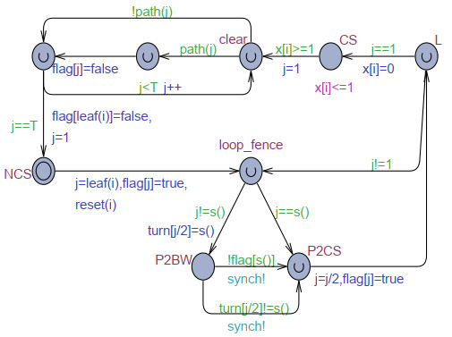
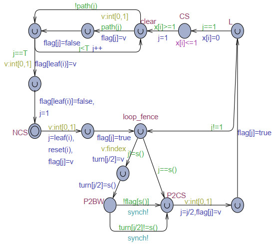
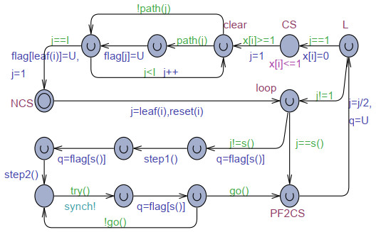
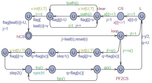
The goal of this work was to experiment with the formal modeling and automated reasoning of concurrent/parallel systems, mainly focusing on mutual exclusion algorithms. A concrete method is presented, which depends on timed automata and the model checker provided by the popular Uppaal toolbox. The method can be used for a thorough assessment of the properties of mutual exclusion algorithms. The paper argues that the proposed approach can be effective in moving beyond informal and intuitive reasoning about concurrency, which can be challenging due to the non-determinism and interleaving of the action execution order of the involved processes. The approach is described and applied to an in-depth analysis of Peterson's algorithms for $ N = 2 $ and $ N > 2 $ processes. The analysis allows the reconciliation of different evaluations reported in the literature, particularly for the overtaking bound, and also reveals new results not previously disclosed. The general case of $ N > 2 $ was handled within the context of the state-of-art, standard, and efficient tournament binary-tree organization, which uses the solution for two processes to arbitrate between pairs of processes at different stages of their upward movement along the tree. All mutual exclusion algorithms are investigated under both atomic and non-atomic memory models.
- mutual exclusion problem,
- safety and liveness properties,
- memory models,
- formal modeling,
- model checking,
- timed automata,
- Uppaal,
- Java
Citation: Libero Nigro, Franco Cicirelli. Property assessment of Peterson's mutual exclusion algorithms[J]. Applied Computing and Intelligence, 2024, 4(1): 66-92. doi: 10.3934/aci.2024005

Related Papers:

Abstract

The goal of this work was to experiment with the formal modeling and automated reasoning of concurrent/parallel systems, mainly focusing on mutual exclusion algorithms. A concrete method is presented, which depends on timed automata and the model checker provided by the popular Uppaal toolbox. The method can be used for a thorough assessment of the properties of mutual exclusion algorithms. The paper argues that the proposed approach can be effective in moving beyond informal and intuitive reasoning about concurrency, which can be challenging due to the non-determinism and interleaving of the action execution order of the involved processes. The approach is described and applied to an in-depth analysis of Peterson's algorithms for $ N = 2 $ and $ N > 2 $ processes. The analysis allows the reconciliation of different evaluations reported in the literature, particularly for the overtaking bound, and also reveals new results not previously disclosed. The general case of $ N > 2 $ was handled within the context of the state-of-art, standard, and efficient tournament binary-tree organization, which uses the solution for two processes to arbitrate between pairs of processes at different stages of their upward movement along the tree. All mutual exclusion algorithms are investigated under both atomic and non-atomic memory models.

References

[1]	E. W. Dijkstra, Co-operating sequential processes, In: The origin of concurrent programming, New York: Springer, 1968, 65–138. https://doi.org/10.1007/978-1-4757-3472-0_2
[2]	M. Raynal, D. Beeson, Algorithms for mutual exclusion, Cambridge: MIT Press, 1986.
[3]	A. Silbershatz, P. N. Galvin, G. Gagne, Operating system concepts, 10 Eds., New Jersey: John Wiley & Sons, Inc., 2018.
[4]	E. W. Dijkstra, Solution of a problem in concurrent programming control, Commun. ACM, 8 (1965), 569. https://doi.org/10.1145/365559.365617 doi: 10.1145/365559.365617
[5]	G. L. Peterson, Myths about the mutual exclusion problem, Inform. Process. Lett., 12 (1981), 115–116. https://doi.org/10.1016/0020-0190(81)90106-X doi: 10.1016/0020-0190(81)90106-X
[6]	E. M. Clarke, O. Grumberg, D. Kroening, D. A. Peled, H. Veith, Model checking, Cambridge: MIT Press, 2018.
[7]	C. Baier, J. P. Katoen, Principles of model checking, Cambridge: MIT Press, 2008.
[8]	G. Behrmann, A. David, K. G. Larsen, A tutorial on UPPAAL, In: M. Bernardo, F. Corradini (Eds.), Formal methods for the design of real-time systems, Berlin: Springer, 2004,200–236. https://doi.org/10.1007/978-3-540-30080-9_7
[9]	F. Cicirelli, A. Furfaro, L. Nigro, Model checking time-dependent system specifications using time stream Petri nets and Uppaal, Appl. Math. Comput., 218 (2012), 8160–8186. https://doi.org/10.1016/j.amc.2012.02.018 doi: 10.1016/j.amc.2012.02.018
[10]	L. Nigro, F. Cicirelli, Formal modeling and verification of embedded real-time systems: an approach and practical tool based on constraint time Petri nets, Mathematics, 12 (2024), 812. https://doi.org/10.3390/math12060812. doi: 10.3390/math12060812
[11]	M. Hofri, Proof of a mutual exclusion algorithm – a 'Class'ic example, ACM SIGOPS Operating Systems Review, 24 (1990), 18–22. https://doi.org/10.1145/90994.9100 doi: 10.1145/90994.9100
[12]	T. Kowalttowski, A. Palma, Another solution of the mutual exclusion problem, Inform. Process. Lett., 19 (1984), 145–146. https://doi.org/10.1016/0020-0190(84)90093-0 doi: 10.1016/0020-0190(84)90093-0
[13]	L. Nigro, F. Cicirelli, F. Pupo, Modeling and analysis of Dekker-based mutual exclusion algorithms, Computers, 13 (2024), 133. https://doi.org/10.3390/computers13060133 doi: 10.3390/computers13060133
[14]	L. Nigro, F. Cicirelli, Correctness verification of mutual exclusion algorithms by model checking, Modelling, 5 (2024), 694–719. https://doi.org/10.3390/modelling5030037 doi: 10.3390/modelling5030037
[15]	L. Nigro, Formal modelling and verification of Lycklama and Hadzilacos's mutual exclusion algorithm, Mathematics, 12 (2024), 2443. https://doi.org/10.3390/math12162443 doi: 10.3390/math12162443
[16]	E. A. Lycklama, V. Hadzilacos, A first-come-first-served mutual-exclusion algorithm with small communication variables, ACM Trans. Progr. Lang. Sys., 13 (1991), 558–576. https://doi.org/10.1145/115372.115370 doi: 10.1145/115372.115370
[17]	A. A. Aravind, Simple, space-efficient, and fairness improved FCFS mutual exclusion algorithms, J. Parallel Distr. Com., 73 (2013), 1029–1038. https://doi.org/10.1016/j.jpdc.2013.03.009 doi: 10.1016/j.jpdc.2013.03.009
[18]	J. Burns, Complexity of communication among asynchronous parallel processes, Ph. D. Thesis, Georgia Institute of Technology, 1981.
[19]	L. Lamport, The mutual exclusion problem: part Ⅱ: statement and solutions, JACM, 33 (1986), 313–348. https://doi.org/10.1145/5383.5385 doi: 10.1145/5383.5385
[20]	R. Alur, D. L. Dill, A theory of timed automata, Theor. Comput. Sci., 126 (1994), 183–235. https://doi.org/10.1016/0304-3975(94)90010-8 doi: 10.1016/0304-3975(94)90010-8
[21]	Uppaal on-line, Uppsala University and Aalborg University, June 2024. Available from: https://uppaal.org.
[22]	E. M. Clarke, W. Klieber, M. Nováček, P. Zuliani, Model checking and the state explosion problem, In: Tools for practical software verification, Berlin: Springer, 2011, 1–30. https://doi.org/10.1007/978-3-642-35746-6_1
[23]	P. A. Buhr, D. Dice, W. H. Hesselink, Dekker's mutual exclusion algorithm made RW‐safe, Concurr. Comp.-Pract. E., 28 (2016), 144–165. https://doi.org/10.1002/cpe.3659 doi: 10.1002/cpe.3659
[24]	L. E. Frenzel, Dual-port SRAM accelerates smart-phone development, Electron. Des., 4 (2004), 35.
[25]	G. L. Peterson, M. J. Fischer, Economical solutions for the critical section problem in a distributed system, Proceedings of the ninth annual ACM symposium on Theory of computing, 1977, 91–97. https://doi.org/10.1145/800105.803398 doi: 10.1145/800105.803398
[26]	J. L. W. Kessels, Arbitration without common modifiable variables, Acta Inform., 17 (1982), 135–141. https://doi.org/10.1007/BF00288966 doi: 10.1007/BF00288966
[27]	W. H. Hesselink, Tournaments for mutual exclusion: verification and concurrent complexity, Form. Asp. Comp., 29 (2017), 833–852. https://doi.org/10.1007/s00165-016-0407-x doi: 10.1007/s00165-016-0407-x
[28]	X. Ji, L. Song, Mutual exclusion verification of Peterson's solution in Isabelle/HOL, Proceedings of Third International Conference on Trustworthy Systems and their Applications, 2016, 81–86. https://doi.org/10.1109/TSA.2016.22 doi: 10.1109/TSA.2016.22
[29]	W. Hesselink, Correctness and concurrent complexity of the Black-White Bakery algorithm, Form. Asp. Comp., 28 (2016), 325–341. https://doi.org/10.1007/s00165-016-0364-4 doi: 10.1007/s00165-016-0364-4
[30]	Y. Hafidi, J. J. Keiren, J. F. Groote, Fair mutual exclusion for N processes, In: Tools and methods of program analysis, Cham: Springer, 2021,149–160. https://doi.org/10.1007/978-3-031-50423-5_14
[31]	T. Murata, Petri nets: properties, analysis and applications, Proc. IEEE, 77 (1989), 541–580. https://doi.org/10.1109/5.24143 doi: 10.1109/5.24143
[32]	L. Nigro, Parallel theatre: an actor framework in Java for high performance computing, Simul. Model. Pract. Th., 106 (2021), 102189. https://doi.org/10.1016/j.simpat.2020.102189 doi: 10.1016/j.simpat.2020.102189
[33]	L. Nigro, F. Cicirelli, P. Fränti, Parallel random swap: an efficient and reliable clustering algorithm in Java, Simul. Model. Pract. Th., 124 (2023), 102712. https://doi.org/10.1016/j.simpat.2022.102712 doi: 10.1016/j.simpat.2022.102712

Reader Comments

Your name:*

Email:*
© 2024 the Author(s), licensee AIMS Press. This is an open access article distributed under the terms of the Creative Commons Attribution License (http://creativecommons.org/licenses/by/4.0)